
Quick Answer
A load line plots every combination of device voltage and device current a supply and its series resistance will allow, as a straight line on the device's own axes. Where that line crosses the device's characteristic is the operating point, and it satisfies both constraints at once.
Intuition
The price the buyer will pay, and the price the seller will take
Listen to two parties haggling. One will pay more only if less is supplied; the other will supply more only if paid more. Neither statement decides anything on its own, and neither is negotiable. Draw both as lines on the same pair of axes and there is exactly one place they meet, and that is where the deal lands.
A device and its load are in that position. The device says what current a given voltage across it will produce — that is its characteristic, and it belongs to the part rather than to the circuit. The load says what voltage will be left over once a given current has flowed through it — that is Ohm's law applied to the resistor and the supply, and it belongs to the circuit rather than to the part.
Put both on the same axes and the crossing is the answer. It has to be, because it is the only pair of numbers that satisfies both.
The method is worth learning for two separate reasons. For a nonlinear device like a diode there is no tidy algebra, and the graphical crossing is often the clearest way to get an honest number. For a transistor there is no single crossing at all — the device has a whole family of curves, one per drive level — and the load line turns "how much drive" into "where on this line do I want to sit", which is a much better question.
Practitioner
Drawing the line, and using it on something nonlinear
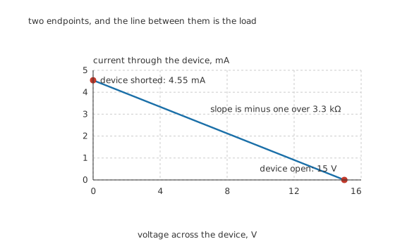
Two endpoints, and the line between them is everything the load permits.
The construction takes two points and no more.
Worked example — The two endpoints, and what they mean
If the device were a dead short, all of 15 V would appear across 3.3 kΩ and the current would be 4.55 mA. That is the line's intercept on the current axis.
If the device were an open circuit, no current would flow and the whole 15 V would stand across the device. That is its intercept on the voltage axis.
Join them. The slope is minus one over 3.3 kΩ, and nothing about the device has been used yet — a different device on the same load draws exactly the same line.
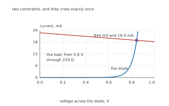
Two constraints, and they cross exactly once.
Worked example — Solving a diode without algebra
Take a diode that passes 1.0 mA at 0.70 V, with an ideality of 1.9, fed from 5.0 V through 220 Ω.
The device's curve and the load's line cross at 844 mV and 18.9 mA. That is the circuit's answer, and it required no rearranging of an exponential.
Engineer
What the shortcut costs, and how the method changes for a transistor
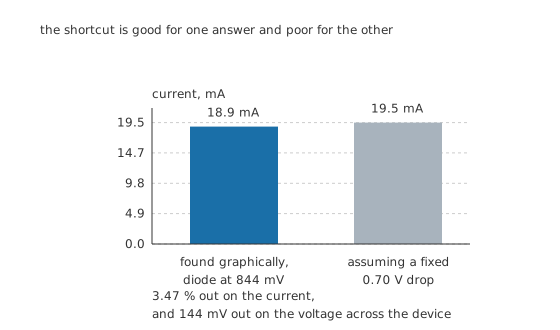
The shortcut is good for one answer and poor for the other.
Worked example — Checking the constant-drop assumption against the crossing
The usual shortcut assumes a fixed 0.70 V across the diode and does the arithmetic in one line, giving 19.5 mA.
Against the true 18.9 mA that is 3.47 % high — close enough for most purposes, because the resistor is dropping most of the supply and a hundred millivolts hardly moves it.
The voltage is where the shortcut fails. The real drop is 144 mV above the assumed one. Any calculation that needed the device's own voltage — a level shift, a reference, a temperature measurement — has been answered wrongly by a shortcut that answered the current well.
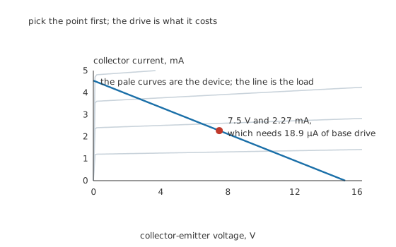
Pick the point first; the drive is what it costs.
A transistor changes the exercise in one respect. It does not have a characteristic; it has a family of them, one for each base current. Every curve in that family crosses the load line once, so the load line becomes a menu rather than a solution.
Worked example — Choosing a point, and reading off what it demands
Sitting halfway along the line puts the device at 7.5 V, which by the load line means 2.27 mA is flowing.
With a gain of 120, that current needs 18.9 µA of base drive.
The arrow runs that way round and it matters. Choosing a drive and finding out where the device lands is how a circuit ends up saturated or cut off; choosing the point and computing the drive it costs is what biasing is.
Professional
The second line nobody draws, and the swing it steals
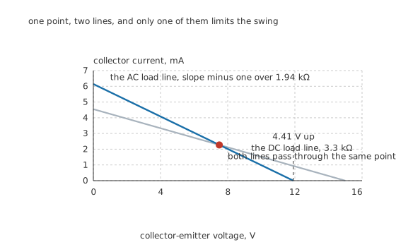
One point, two lines, and only one of them limits the swing.
Here is the part that catches people. A stage with a coupled load has two load lines, and they are not the same.
Worked example — Why the DC picture overstates the swing
For DC, the collector sees only 3.3 kΩ, because the coupling capacitor blocks everything. That is the line the bias sits on.
For signals the capacitor is a short, so the collector sees 3.3 kΩ and 4.7 kΩ in parallel — 1.94 kΩ. The signal therefore moves along a steeper line through the same point.
The DC picture suggests the output could fall 7.30 V before saturating. The AC line runs out first: the quiescent 2.27 mA flowing into 1.94 kΩ can only produce 4.41 V of swing before the collector current has all been diverted and the device cuts off.
4.41 V is the honest figure and 7.30 V is the flattering one, and a stage designed on the flattering one clips on one side at about two-thirds of its expected output.
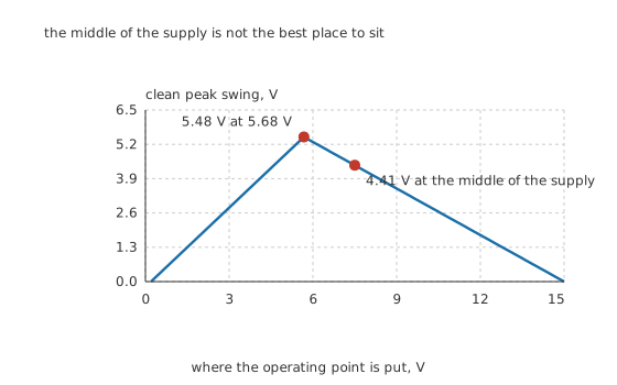
The middle of the supply is not the best place to sit.
Worked example — Moving the point to where the two limits are equal
Since one limit rises as the point moves down the line and the other falls, the best place is where they are equal — taking the device down to a saturation voltage of 0.20 V at one extreme. Solve for it and the point lands at 5.68 V with 2.83 mA flowing, needing 23.5 µA of base drive.
The clean swing there is 5.48 V, against 4.41 V at mid-supply.
24.3 % more output, from the same supply, the same load, the same device and the same standing power. Only the bias resistor values changed.
Four places the method earns its keep
Any device with a published curve and no usable equation. Thermistors, varistors, lamps, photodiodes into a load, and the whole family of parts characterised by a graph rather than a formula. The load line is often the only honest way to read an operating point off them.
Sanity-checking a simulation. Two intercepts and a straight edge take a minute and catch the class of error where a supply, a resistor or a decimal point is wrong. A simulator will confidently report a transistor operating at more current than the load could ever pass.
Understanding what saturation and cut-off actually are. They are simply the two ends of the line — the point running off one edge of the useful region. Seeing them as positions rather than as states makes the regions obvious.
Deciding whether a resistive load is the right load at all. The AC line's slope is what limits the swing, and replacing the collector resistor with a current source makes that line almost horizontal, which is why integrated amplifiers do it and resistor-loaded discrete stages cannot compete on either gain or swing.
Two limits of the construction
It is a DC and low-frequency picture. Nothing on these axes accounts for capacitance, so the load line says nothing about what happens at frequencies where the device's own reactances matter.
It assumes the load is a resistance. An inductive load — a relay coil, a motor winding, a transformer primary — traces an ellipse rather than a line, and the device can end up at combinations of voltage and current that no straight line would ever have predicted. That is the reason a safe operating area is drawn as a region rather than a line.
Common mistakes
- Choosing the drive first and hoping — the load line runs the other way. Pick where the device should sit, read off the current, and work out what drive that costs: 18.9 µA for a point at 7.5 V here.
- Forgetting the AC load line — a coupled load puts a steeper line through the same point. The DC picture promises 7.30 V of downward swing and the AC line delivers 4.41 V.
- Sitting at mid-supply out of habit — with this load, moving the point to 5.68 V raises the clean swing from 4.41 V to 5.48 V, which is 24.3 % more for nothing.
- Trusting a constant-drop model for the device's own voltage — it gets the current within 3.47 % here and the diode voltage wrong by 144 mV.
- Drawing the line from the device's data — the line comes from the supply and the resistor alone. If the device changed anything about it, it would not be a constraint the device has to satisfy.
Frequently asked questions
How do I draw a load line?
Two points. Assume the device is a short: the current is the supply divided by the load resistance, 4.55 mA here. Assume it is open: the voltage across it is the whole supply, 15 V. Join them. The slope is minus one over the load resistance, and nothing about the device enters it.
Why bother when I could just do the algebra?
For a resistor you can. For an exponential device the algebra does not rearrange, and for a transistor there is no single answer to rearrange towards — the family of curves means the question is which point to choose, not what the point is. The construction handles both.
What is the difference between the DC and AC load lines?
The DC line uses the collector resistor alone and sets the bias. The AC line uses the collector resistor in parallel with the coupled load — 1.94 kΩ here against 3.3 kΩ — so it is steeper and passes through the same operating point. The steeper line is what limits the signal swing.
Where should the operating point go for the largest output?
Where the two limits are equal: where the current available equals the voltage available divided by the AC load. That lands at 5.68 V and 2.83 mA here, giving 5.48 V of clean peak swing against 4.41 V at mid-supply — 24.3 % more.
Does the load line work for anything other than transistors and diodes?
Any two-terminal device whose behaviour is a curve on the current-voltage plane, which is most of them. Thermistors, lamps, varistors and photodiodes are all commonly solved this way, and the construction is identical: the line comes from the supply and the resistance, the curve comes from the part.