
Quick Answer
SPICE is a circuit simulator that reads a netlist, meaning a list of components and the two nodes each one joins, then writes one current balance equation per node and solves them numerically. It reports node voltages and branch currents for a fixed operating point, a swept input, or a run through time.
Intuition
A circuit reduced to a list of connections
Most of what a schematic shows is drawn for the person reading it. Where a part sits on the page, how the wires are routed and which way a symbol faces all belong to that reader. The program takes something narrower from the same sheet: which parts join which points. That much is the circuit.
So the drawing becomes a list. Each entry names one component, the two points it connects, and its value. Those points are called nodes and are given numbers, and one number is reserved: node 0 is the reference that every voltage in the answer is measured against — the ground of the analysis.
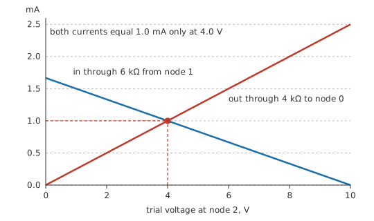
Take a source of 10 V sitting between node 1 and node 0, a resistor of 6 kΩ between node 1 and node 2, and a resistor of 4 kΩ between node 2 and node 0. Those entries describe the circuit completely. Node 1 is held at the supply and node 0 is the reference, so one unknown is left, the voltage at node 2. The program finds it by requiring that the current arriving at node 2 through the upper resistor is the same current that leaves through the lower one. Only one value satisfies that: 4.0 V, with 1.0 mA in both resistors.
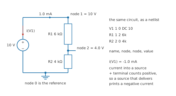
A larger circuit changes the size of that problem rather than its shape. The unknowns are the node voltages, and the equations come from insisting that current balances at each node, so what comes back is a table of numbers. Waveforms and curves are drawn afterwards from those numbers.
Practitioner
Netlist, node numbers, first run
A netlist entry is short. R1 1 2 15k is a resistor called R1 joining node 1 to node 2; V1 1 0 DC 12 is a voltage source whose positive terminal is at node 1 and whose negative terminal is at node 0. The first letter of the name says what kind of part it is, the nodes come next, and the value or model name comes last.
Typing them by hand is instructive on a circuit of five parts and unbearable on one of five hundred, so most work is done in a schematic editor that generates the same list from a drawing. Knowing what it generates is what lets you read the list back and see that a symbol left a grid square short of a wire produced a circuit you did not draw. Schematic symbols and the netlist generated from them are one circuit written down two ways.
Node numbers are labels and carry no meaning beyond identity. Node 0 is the exception and is not optional, since it is the origin every other node voltage is quoted from.
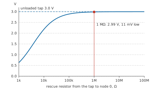
Far more often the trouble is a node that exists but has no conducting path to node 0 at DC, and it announces itself less clearly. Its voltage is then undetermined, the equations have no unique solution, and the run stops with a complaint about a floating node or a singular matrix. A capacitor between two stages does it, since no DC current passes through a capacitor. So does a transformer winding, an op-amp input left unconnected, or a subcircuit whose ground pin was never joined to anything. The cure is to supply the missing path on purpose, usually a resistor from the orphaned node to the reference, large enough to change nothing else.
The analyses to reach for first
An operating point holds every source at its DC value and solves the circuit once, which gives the steady state: one voltage per node, one current per source. It is where a DC circuit belongs, and where an investigation of anything else should start.
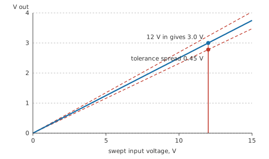
Step one source through a range, re-solving the operating point at every value, and you have a DC sweep, with a chosen output plotted against the swept input. Sweep the supply of the divider above from zero upwards and the tap traces a straight line rising 0.25 volts per volt of input. Transfer characteristics, bias points and switching thresholds come out of this one.
A transient run starts from an initial state and steps the circuit forward in time, so capacitors and inductors behave as they do on a bench. Waveforms come from here, and so does anything with energy storage in it.
A first DC run, in order
- Write the netlist, or draw the schematic that will generate it. Either way, the deliverable is a list of components and connections.
- Name the nodes. Every junction gets one label. Two points joined by a wire are one node however far apart they sit on the page.
- Set the reference. Choose the point that every voltage should be quoted against, normally the supply's negative terminal, and make it node 0.
- Check that every node has a DC path back to node 0. Follow it through resistors, sources and windings; capacitors do not count.
- Give every part a usable value or model. A part with no value and a model name the simulator cannot resolve will stop the run before any arithmetic happens.
- Work out by hand what the answer should be, and write it down. For a resistive circuit this is a divider ratio and a current, and it takes a minute.
- Ask for an operating point. A single analysis, with the sweep and the time axis left for later.
- Run it and read the node voltage table and the source currents. These are the primary output; anything plotted is derived from them.
- Compare every number against step 6. Agreement means the netlist is the circuit you meant and your analysis of it holds.
- Change one thing and repeat. When a disagreement follows a single change, that change is where to look; alter three things together and the reading has nothing to say about any of them.
Step 6 is the one people skip. Without it the simulator is being consulted rather than checked, and its answer has nothing to stand against. For a chain of two resistances between a rail and the reference, the junction sits in proportion to the arms:
and the current in that chain is the supply across the sum of the two:
Worked example — Predicting the result before running it
Take the netlist above in full: 12 V from node 1 to node 0, 15 kΩ from node 1 to node 2, 5 kΩ from node 2 to node 0.
Both resistors carry one current, so node 2 sits at the supply scaled by the lower arm over the sum of the arms, which is 3.0 V. That same current is the supply divided by the sum of the arms, 0.6 mA.
The operating point should therefore report node 1 at 12 V, node 2 at 3.0 V, and a source current of -0.6 mA. The minus sign comes from a sign convention: SPICE counts current flowing into a source's positive terminal as positive, so a source delivering power into a circuit reports a negative figure — here 0.6 mA in magnitude.
Write those numbers down before the run and the run becomes a test of the netlist and of the hand analysis together. A disagreement puts one of the two in the wrong, and on a circuit this small either is cheap to find. On a circuit of two hundred parts the search costs a great deal more, which is the argument for doing this while the circuit is still small.
Going deeper
Convergence, models and ratings
When the solver gives up
Resistive circuits give linear equations, and linear equations are solved once and exactly. Diodes, transistors and anything else with a curved characteristic do not. For those the solver guesses an operating point, replaces each nonlinear device with a straight-line approximation valid near the guess, solves the resulting linear circuit, and takes that answer as the next guess. It repeats until two successive answers differ by less than a set tolerance. A convergence failure says that the sequence never settled inside the iteration limit. The complaint is about the search, and the circuit itself has yet to be judged at all.
The usual causes are structural. A node without a DC path to the reference has no unique solution to converge to. Wholly ideal elements make the equations badly behaved: a source of exactly zero resistance across an ideal switch, or two ideal sources in one loop, describe a situation with no finite answer. Some circuits genuinely have no stable operating point, or several, and a bistable circuit given no starting hint has no reason to prefer either. In a transient run, time constants spread across many decades force the solver into very small steps and can exhaust its patience before the interesting part of the waveform arrives.
Putting back what the idealisation left out cures most of them: the small resistances real parts have — source resistance, switch on-resistance, winding resistance — and a large resistor from any floating node to the reference. Supply an initial guess for the nodes you know, or ramp the supplies from zero so the solver walks to the answer instead of jumping to it. Loosening tolerances or raising the iteration limit is the last resort, and a circuit that only converges after that treatment deserves another look at its topology before its results are believed.
The model is a set of numbers someone chose
Every device in a simulation is an equation with parameters in it, and the answer inherits whatever those parameters happen to describe. A resistor holds its value at any temperature unless a coefficient is entered for it. A semiconductor model was fitted to measurements of particular samples from a particular process, so the manufacturer's model for the exact part is the one to use. One borrowed from something roughly similar may put the operating point in the right place and every second-order detail in the wrong one.
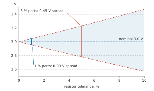
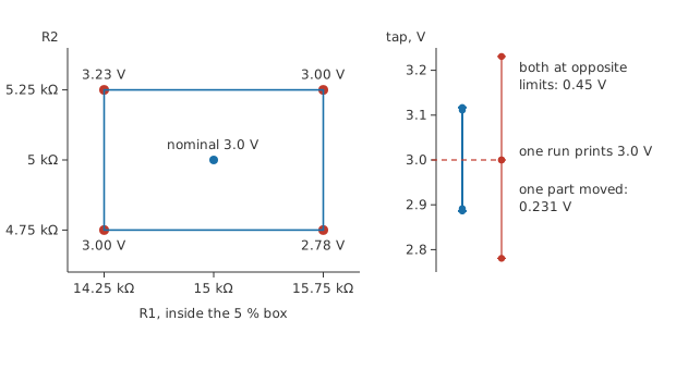
Tolerance is absent unless it is asked for, and of all the gaps this is the quietest. The divider worked through above prints 3.0 V to as many decimal places as you care to request. Built from 5 % parts, its arms may sit at 14.25 kΩ over 5.25 kΩ, which puts the tap at 3.23 V; the opposite corner, 15.75 kΩ over 4.75 kΩ, gives 2.78 V. A real production run is spread across 0.45 V, and the printed answer sits in the middle of that spread reporting none of it. Declaring the tolerances and asking for a sweep across them, or a Monte Carlo run, turns the nominal answer into a distribution, and the distribution is what the boards will actually do.
Ratings are outside the equations
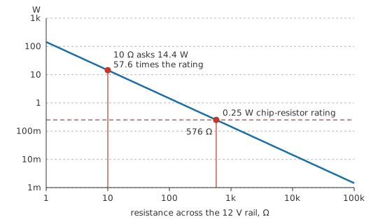
The solver works in currents and voltages, and maximum dissipation, working voltage, track width and ambient temperature are nowhere in its equations. Put 12 V across 10 Ω and the report comes back 1.2 A and 14.4 W: correct arithmetic, delivered without comment. A common 0.25 W chip resistor in that position is being asked for 57.6 times what it can shed, and it will not last the minute. The same silence covers capacitor working voltage, transistor safe operating area, connector current, creepage across a board and every mechanical fact about the assembly. Checking power dissipation element by element against each part's power rating is a separate pass, and the engineer is the one who makes it.
Every one of those gaps is a reason to read the output carefully rather than a reason to leave the simulator switched off. It answers questions a bench answers slowly or not at all: the current in a node you cannot reach with a probe, the behaviour at both corners of a tolerance band, a hundred variations of one component value before a single part is bought. What it returns is the consequence of the netlist and the models it was handed, and it answers that question well. A hand calculation first and a measured board afterwards are what turn it into evidence.
Safety
Safety is a separate assessment, and no simulation carries it out. Isolation, clearance and creepage distances, insulation ratings, fusing, earthing and enclosure all sit outside the equations a solver handles, and a circuit that behaves impeccably on screen can still be unsafe to build and unsafe to power. Anything intended to connect to mains or to hold significant stored energy needs the working practices in electrical safety fundamentals applied to the physical build, whatever the simulation showed.
Common mistakes
- A node with no DC path to the reference. Coupling capacitors, transformer windings and unconnected subcircuit pins all leave one behind, and the run stops on a floating node or a singular matrix. Add a large resistor from that node to node 0.
- "It simulated fine, so the hardware will work." The simulation confirms that the netlist you supplied, with the models you supplied, produces those numbers. Ratings, layout, tolerance spread, temperature and assembly are untouched by it.
- Decimal places read as accuracy. An output quoted to six figures reports the precision of the solver, while the uncertainty of the circuit sits in the parts. Their tolerance has to be entered before it can appear.
- Two points joined on the drawing but not in the netlist — a wire ending near a pin instead of on it. The schematic looks right and the simulation is of a different circuit. Reading the generated netlist back is the check.
- A model borrowed from a part that seemed close enough. Substituted models are useful for a first look and misleading in the details. Where the result matters, use the manufacturer's model for the part actually being fitted.
- Convergence bought by loosening tolerances. Raising the iteration limit and relaxing the error targets can make a run finish without making its answer trustworthy. Find the ideal element or the floating node first.
Frequently asked questions
What does SPICE stand for?
Simulation Program with Integrated Circuit Emphasis. It began as an academic program at Berkeley and its netlist syntax, analysis commands and device models became the common language of circuit simulation, which is why so many later tools describe themselves as SPICE-compatible.
Why does my netlist need a node 0?
Voltages are differences, so the solver needs one point declared as the origin before any other node voltage means anything. SPICE reserves node 0 for that purpose. Without it there is no fixed reference, the equations have no unique solution, and the run stops before it starts.
What does a convergence error actually mean?
The solver iterates towards the operating point of a nonlinear circuit, and a convergence error says the iterations never settled within its limits. It is a statement about the numerical process. Very often the underlying cause is a genuine modelling problem — a floating node, a perfectly ideal element, or a circuit with no single stable answer.
Which analysis should I run first?
An operating point, almost always. It is the cheapest run, it tells you where every node sits with the sources at their DC values, and a wrong operating point makes every sweep and every waveform after it wrong as well. Move on to a DC sweep or a transient once the DC picture matches expectation.
Does a simulation replace building the circuit?
No. The arithmetic is rarely where it falls short: layout, parasitics, part tolerance, temperature, assembly faults and every rating live outside the model. Simulation is best used to choose between designs and to explore a circuit cheaply, and a built and measured prototype is what confirms one.