
Quick Answer
A 10x oscilloscope probe puts a resistance in series with the scope's input to divide the signal by ten. That division costs amplitude and buys a tenfold reduction in the capacitance the circuit has to drive, and a trimmer inside the probe has to be set so the division holds at every frequency.
Intuition
The probe is part of the circuit
A probe looks like a wire with a hook on it. Electrically it is a component, and on any fast or high-impedance signal it is the component that decides what the trace looks like.
The scope's input is a resistance and a capacitance in parallel, typically 1.00 MΩ and 20.0 pF. Reach that input through a plain lead and the cable adds capacitance of its own, around 100 pF for a metre of coaxial cable, so the circuit under test has to charge and discharge the whole lot on every edge. That is what a 1x probe presents.
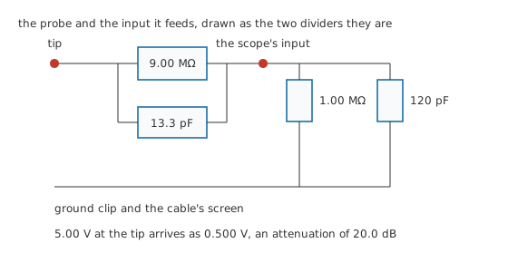
A 10x probe puts 9.00 MΩ in series with the tip. The signal now meets a divider: 9.00 MΩ against the scope's 1.00 MΩ, so a tenth of it reaches the input and nine tenths is dropped in the probe. What that buys is capacitance, because the same series element separates the tip from the cable, and Layer 3 does the arithmetic.
The trade is worth taking almost always, and it has a price. A tenth of the signal reaches the scope, so a small signal gets smaller and the scope's own noise stays where it was. And the division only stays at ten to one across frequency if the probe is adjusted to the particular input it is plugged into.
Spectacles with the wrong prescription are the right picture to hold onto. Everything is still there, in the right place and roughly the right size. The edges are wrong, and until someone tells you, they look like the edges of the thing you are looking at.
Practitioner
Choosing between 1x and 10x
The default is 10x; know the exceptions before you reach for the switch.
- Use 10x unless the signal is too small for it. The probe loads the circuit ten times less, and on anything with an edge in it that is the difference between measuring the circuit and measuring the probe.
- Use 1x when the signal is small and slow. A few millivolts of audio on a low-impedance node needs the amplitude more than it needs the light loading.
- Set the scope's attenuation menu to match the probe. Modern probes tell the scope automatically through an extra ring on the connector; older ones do not, and a scope set for 1x with a 10x probe fitted reads ten times low with nothing on the screen to say so.
- Compensate the probe on the channel you will use it on, every time you move it between channels or instruments. Layer 3 explains what the adjustment does.
- Use the shortest ground return the probe offers. The clip-on lead is convenient and it is also an inductor.
- Put the ground return on the circuit's reference near the point you are probing, not on a distant chassis screw.
The division itself is the ordinary two-resistor relationship:
and expressing it in decibels gives the number a datasheet is likely to quote:
Worked example — What reaches the screen
The probe's 9.00 MΩ and the scope's 1.00 MΩ put 10.0 MΩ between the tip and the scope's own ground, and divide whatever arrives.
A signal of 5.00 V at the tip therefore reaches the input as 0.500 V, which is 20.0 dB of attenuation. The scope multiplies the reading back up by ten before displaying it, which is why the screen shows the right number as long as the attenuation menu agrees with the probe fitted.
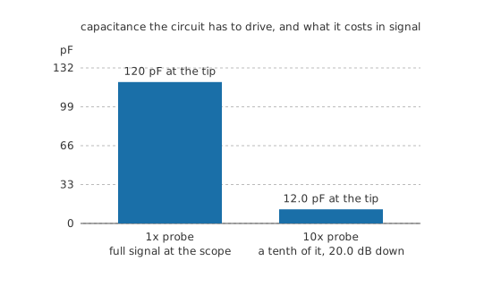
That factor of ten is a loss of signal and a gain of nothing until you look at what the tip presents to the circuit, which Layer 3 works out at 12.0 pF against the 120 pF a 1x probe would hang there.
Safety
The probe's ground clip is joined to the scope's chassis and, on a mains-powered instrument, to the protective earth of the building. Clipping it to a point that is not at earth potential connects that point to earth through the probe lead.
That hazard belongs to the instrument rather than to the probe, and using an oscilloscope sets it out in full, along with the differential and isolated probes that answer it. It is repeated here only because this lesson spends its time on where the ground clip should go, and the answer changes completely on mains-referenced equipment.
One more point: a probe carries a voltage rating, and it is not the same as the scope's. Exceeding it puts the signal through the probe body and into your hand.
Engineer
Compensation, and what happens when it is wrong
The resistive divider is only half of the probe. Capacitance sits across each arm, and at any frequency where those capacitances matter they form a divider of their own. Two dividers in parallel that disagree with each other give a ratio that depends on frequency, which turns a square wave into something else.
Making them agree is what the trimmer in every 10x probe is for. The condition is that the two arms have equal time constants:
The far arm is the scope's 20.0 pF plus the cable's 100 pF:
which comes to 120 pF. The trimmer must therefore be set to 13.3 pF, a ninth of that, matching the ninefold difference in the resistive arms.
What the tip presents once it is matched
With the trimmer set, the tip sees the compensation capacitance in series with everything beyond it:
giving 12.0 pF, a tenth of the 120 pF a 1x probe would put there. The trade sums up the 10x probe entirely: a tenfold loss of amplitude in exchange for a tenfold reduction in what the circuit has to charge.
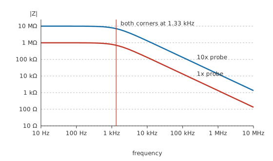
The two probes have the same corner frequency, which surprises people. The 10x probe is 10.0 MΩ shunted by 12.0 pF; the 1x probe is 1.00 MΩ shunted by 120 pF. Both products are the same, so:
gives 1.33 kHz for either. What differs is the impedance at every frequency, which is a decade higher for the 10x probe from one end of the axis to the other.
Setting the trimmer, and what a wrong setting looks like
Every scope has a small terminal producing a square wave for this purpose. Clip the probe to it, look at the flat top, and turn the trimmer until it is flat.
The mathematics of the wrong settings is the same first-order response as any RC network. The two arms in parallel are 900 kΩ and their capacitances add to 133 pF:
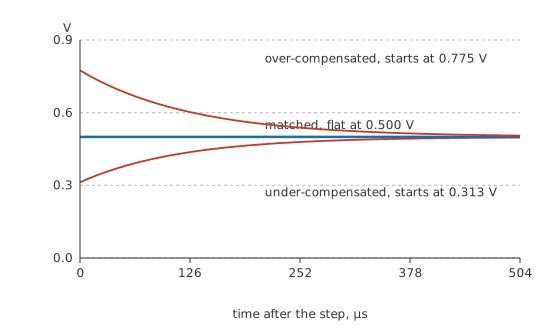
which is 120 µs. At the instant of a step the capacitive divider alone decides the level; long after it, the resistive divider does; and the trace moves exponentially from one to the other:
Set the trimmer to 8.00 pF and the step starts at 0.313 V and climbs to 0.500 V, so every flat top slopes upward and every fast edge is under-reported. Set it to 22.0 pF and it starts at 0.775 V and falls, so edges overshoot and the display flatters the circuit.
The ground lead is an inductor
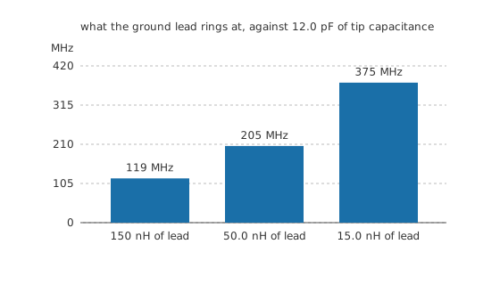
The return path from the ground clip back to the scope has inductance, roughly a nanohenry for each millimetre of lead, and it resonates with the probe's own tip capacitance:
A 150 nH clip lead rings at 119 MHz, so any edge with energy up there arrives at the screen with a decaying oscillation on it that the circuit never produced. The short spring that clips over the probe's barrel is about 15.0 nH and moves the ringing to 375 MHz, above most of what a general-purpose scope can see at all.
What the probe does to an ordinary node
None of this is confined to radio frequencies. Take a node driven through 10.0 kΩ with 22.0 pF of its own, whose edge takes 484 ns unprobed:
A 10x probe adds its 12.0 pF and the edge becomes 748 ns. A 1x probe adds 120 pF instead and it becomes 3.12 µs, more than six times the real figure.
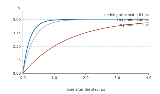
That last trace is a picture of the probe. The circuit is fine, and meter loading effects is the same story told about a meter.
Professional
At the edges of what a passive probe can do
Everything above describes a passive probe, and passive probes run out of usefulness in several directions at once.
Bandwidth is the first. A general-purpose 10x probe is specified at a few hundred megahertz at best, and the specification assumes the short ground spring rather than the clip lead. Above that the probe becomes a transmission line rather than a lumped RC network, and its behaviour depends on how it is terminated. Low-impedance passive probes exist for that region, presenting a few hundred ohms and a fraction of a picofarad, at the cost of loading anything that cannot drive that resistance.
Active probes go further by putting an amplifier at the tip, which gets the input capacitance down to under a picofarad and the resistance up into the megohms at DC and low frequencies. That capacitance is what matters at high frequency: a picofarad is already 159 Ω of reactance at a gigahertz, well below the megohm figure on the label, so what an active probe actually buys at gigahertz frequencies is a far smaller capacitance than any passive probe presents there, not a genuinely resistive input. They need power, they have a limited input voltage range, they cost a great deal, and a moment of carelessness destroys the amplifier rather than blowing a fuse.
Differential probes solve a different problem: measuring between two points where neither is at the scope's ground. That covers a shunt in a high-side current path, a signal on a floating bus, and anything mains-referenced. Their key specification is common-mode rejection, which states how much of a signal common to both inputs leaks into the reading, and it falls with frequency.
Current probes complete the set. A clamp around a conductor senses the magnetic field, using a Hall element for the low-frequency part and a transformer winding for the high-frequency part, and delivers a voltage the scope reads as a current. They load the circuit hardly at all and cost bandwidth, resolution and money in return.
One habit survives all of these. Whatever probe is fitted, the first question about a trace with an unexpected feature on it is whether the feature belongs to the circuit or to the connection. Move the ground return, shorten it, change probes, or take the probe off and watch what a second probe on a neighbouring node does. A feature that changes when you change the probing is a feature of the probing.
Common mistakes
- Leaving the scope's attenuation menu at 1x with a 10x probe fitted. Every voltage on the screen is a tenth of the truth, and the trace looks entirely plausible.
- Compensating a probe once and never again. The adjustment matches the probe to one particular input, and moving it to another channel or another instrument invalidates it.
- Using the long ground clip on a fast edge, then reporting the ringing. A 150 mm lead rings at around a hundred megahertz against the probe's own capacitance, and the circuit had nothing to do with it.
- Reaching for a 1x probe because the signal is small, on a node that is fast or high-impedance. Ten times the capacitance is a heavy price for twice the trace height.
- Grounding at a distant chassis point. The return path is part of the loop, and a long one picks up whatever is passing.
- Treating an overshoot on the screen as a circuit problem before checking the compensation. An over-compensated probe manufactures overshoot on every edge it sees.
Frequently asked questions
Why use a 10x probe when it throws away nine tenths of the signal?
Because the same series resistance separates the tip from the cable and the scope input, cutting the capacitance the circuit has to drive by the same factor of ten. On anything fast or high-impedance that is the difference between measuring the circuit and measuring the probe.
What does compensating a probe actually adjust?
A small trimmer capacitor across the probe's series resistor. Setting it makes the capacitive divider inside the probe match the resistive one, so the division stays at ten to one at every frequency rather than only at DC.
How do I know my probe needs compensating?
Look at the square wave on the scope's own compensation terminal. A sloping or rounded flat top means under-compensated, a peaked one means over-compensated, and flat means correct. Redo it whenever the probe moves to a different channel or instrument.
Why does my square wave ring when I probe a fast circuit?
Usually the ground lead. Its inductance resonates with the probe's tip capacitance, and a typical clip lead rings somewhere around a hundred megahertz. Replace the clip with the short ground spring and the ringing moves above the band you are looking at.
Can I use any 10x probe with any oscilloscope?
Only if its compensation range covers that scope's input capacitance, which is why probes state a range rather than a single value. A probe matched to a 15 pF input may not adjust flat on a 25 pF one, and the probe's bandwidth figure assumes the input it was designed for.