
Quick Answer
An oscilloscope draws a graph of voltage against time on a screen ruled into squares called divisions. You set how many volts one vertical division is worth and how much time one horizontal division covers, and a trigger decides where each sweep begins so the picture stands still.
Intuition
Voltage drawn against time
A multimeter reports one number, averaged over a good fraction of a second. An oscilloscope draws the shape instead, so a signal that rises, falls, rings, glitches or collapses shows all of that on a screen.
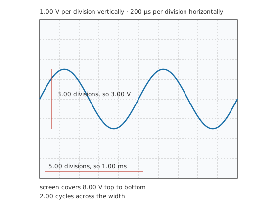
The screen is ruled into a grid, 10 divisions across and 8 down. Two controls give those divisions their meaning. The vertical control says how many volts one division is worth; the timebase says how much time one division covers. Everything else on the front panel exists to make the trace stand still and to point it at the right signal.
Set the vertical to 1.00 V a division and the whole screen covers 8.00 V from top to bottom. Set the timebase to 200 µs a division and the width covers two milliseconds. A 1.00 kHz sine of 3.00 V then stands 3.00 divisions tall and repeats every 5.00 divisions, so 2.00 cycles fill the width and every quantity you want is countable in squares.
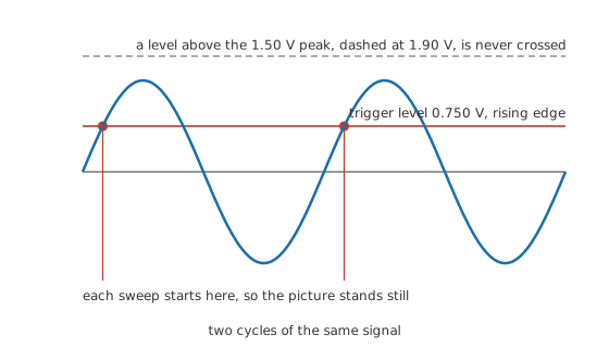
The third control is the one beginners fight with. A sweep across the screen takes a couple of milliseconds and then starts again, and unless every sweep begins at the same point on the waveform the traces land in different places and the picture is a blur. The trigger is what enforces that: it holds the sweep until the signal crosses a level you choose, going the direction you choose. A flip-book only reads as motion if every page is drawn from the same corner, and a trigger is that corner.
Practitioner
Getting a stable trace
Most sessions that end in frustration went wrong in the first thirty seconds. This order avoids that.
- Connect the ground clip first, to the circuit's own reference node, and read the safety notice below before doing it on anything mains-connected.
- Set the coupling to DC unless you already know you want otherwise, so that the trace tells you where zero is.
- Set the vertical roughly, aiming for a trace that fills a good part of the screen without leaving it. Layer 3 shows what a cramped trace costs.
- Set the timebase from the frequency you expect, so that a few cycles fit. Divide the period by five as a starting point.
- Set the trigger source to the channel you are looking at, the slope to rising, and the level somewhere within the signal's swing.
- Use auto trigger while you are hunting and normal trigger once you have found it. Auto sweeps anyway when nothing crosses the level, which shows you something; normal waits, which is what you want for a one-off event.
- Check the probe attenuation setting matches the probe. A scope set for a 1x probe with a 10x probe fitted reads ten times low, and nothing on the screen says so.
The two settings work through one relationship apiece. The period follows from the frequency:
and the number of cycles across the screen is the screen's own width in time divided by that period.
Worked example — Choosing a sweep speed
The signal is 1.00 kHz, so its period is 1.00 ms.
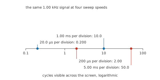
At 200 µs a division, the 10 divisions of screen width cover two milliseconds and hold 2.00 cycles. That is a good working setting: the shape of one cycle is legible and there is a second cycle to confirm the first is repeating.
Speed up to 20.0 µs a division and only 0.200 of a cycle is on screen, which is the setting for looking at one edge and useless for looking at the shape. Slow down to 1.00 ms and 10.0 cycles are squeezed across the width, which shows that the signal is steady and shows nothing about its shape at all.
Safety
The ground clip on a mains-powered scope is connected to the protective earth of the building, and the outer shell of every input connector is joined to it. One consequence of that: clipping the ground lead to a point that is not at earth potential connects that point to earth, through the probe lead and the instrument.
On a battery circuit this does nothing. On mains-connected equipment, and especially on anything transformerless — many switching supplies, motor drives, and most LED drivers — it is a short circuit across part of the mains, and it can put dangerous voltage on the scope's own case and on every other instrument bonded to the same earth.
The correct answers are an isolated or differential probe, or a scope with genuinely isolated inputs. Lifting the scope's own earth pin is not one of them: it removes the protection that keeps the case safe and leaves the case floating at whatever the circuit decides.
Measure the ground clip's intended node against earth with a meter before clipping on, whenever there is any doubt. The general practice for live work is set out in electrical safety fundamentals, and the instrument's own CAT rating states where it may be used at all.
Engineer
Bandwidth, sampling and the signals that lie
A scope has two limits that do not appear anywhere on the front panel, and both of them produce confident, wrong-looking-right pictures.
The front end has its own rise time
Bandwidth is the frequency at which the scope's own response has fallen by three decibels, and for a single-pole front end it fixes the fastest edge the instrument can draw:
A 100 MHz scope therefore has a rise time of 3.50 ns of its own. What appears on the screen is the signal's edge and the scope's edge combined, and for two single-pole stages they combine in quadrature:
A true 10.0 ns edge is reported as 10.6 ns, which is 5.95 % slow and perfectly usable. A true 3.50 ns edge, equal to the scope's own, comes back as 4.95 ns, 41.4 % slow. A true 1.00 ns edge is reported as 3.64 ns, which is 264 % slow and describes the scope rather than the circuit.
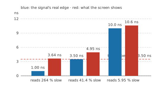
The working rule that falls out of this is to pick a scope whose rise time is comfortably shorter than the edge you care about, which for a five per cent error means about a third of it.
The sample rate invents frequencies
A digital scope takes samples at a fixed rate and draws a curve through them. A signal above half that rate cannot be reconstructed, and what appears instead is a slower signal that fits the same samples exactly.
Sample at 1.00 MHz and the honest limit is 500 kHz. Present a 900 kHz signal and the samples land on a 100 kHz curve, which the scope draws confidently and which never existed.
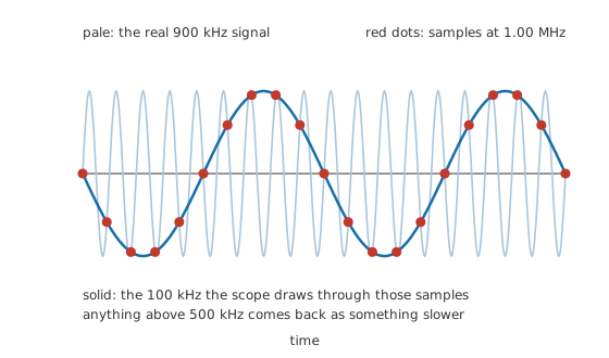
Nothing on the screen distinguishes an alias from a real signal. The defence is to change the timebase: a real frequency stays where it is, and an alias moves, because the sample rate moved with the sweep speed.
Coupling decides what is thrown away
DC coupling passes the signal as it is, steady part included. AC coupling puts a capacitor in the path so only the changing part gets through. That is what makes a small ripple on a large rail measurable at all.
Take 100 mV of ripple on a 5.00 V rail. DC coupled at 2.00 V a division, which is what it takes to keep the rail on screen, the ripple spans 0.0500 of a division and is invisible. AC coupled at 50.0 mV a division, the steady part is gone and the same ripple spans 2.00 divisions.
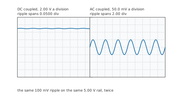
The cost of AC coupling is that zero is no longer on the screen, so a trace that looks centred says nothing about the rail's actual level. It also has a low-frequency limit of its own, which distorts slow square waves by tilting their flat tops.
Counting squares has a width
Reading a value off the graticule by eye is good to something like 0.200 of a division. On the 3.00 V signal at 1.00 V a division, that comes to 6.67 % of the reading. Turn the sensitivity up to 500 mV a division, filling twice as many squares, and the same eye buys 3.33 %.
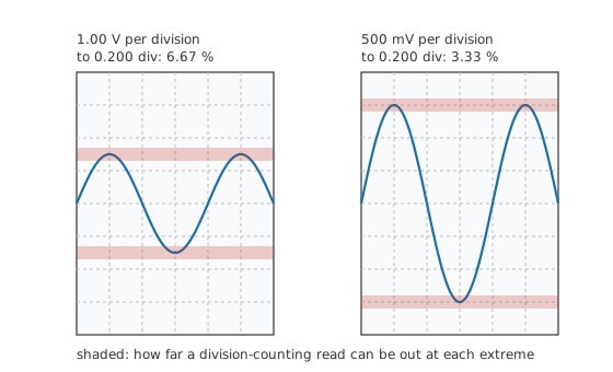
Cursors and automatic measurements remove the eye from the loop and replace its error with the instrument's own, which accuracy, resolution and measurement error sets out. That habit pays off either way.
Professional
What the front panel does not show
Sample rate and memory depth work against each other in a way that catches everyone once. The scope's memory holds a fixed number of samples, so a slow sweep across a long window has to reduce the sample rate to make the record fit. A scope quoting a headline sample rate achieves it only on its fastest timebases, and the same instrument at a slow sweep speed can be sampling slowly enough to alias.
Memory depth is what buys both at once. A deep record lets a scope keep a fast sample rate across a long window, which is what finds a glitch that happens once in a hundred milliseconds without knowing in advance where to look.
Triggering has more to it than a level and a slope. Pulse-width triggers catch a pulse shorter or longer than a stated time, which is how a runt pulse gets found. Serial triggers decode a bus and fire on an address or a data value. Holdoff suppresses re-triggering for a set time after each sweep, which is how a burst gets a stable display when its individual cycles would otherwise each qualify.
The intensity of the trace carries information on an analog scope, where a part of the waveform the beam passes through often is brighter than one it visits rarely. Digital scopes reproduce that deliberately, and it is the difference between seeing a jittery edge and seeing an edge.
Probing is where most real measurement error enters, and it has a lesson of its own. The probe is not a wire: it adds capacitance, it needs compensating to the input it feeds, and its ground lead is an inductor that rings. Oscilloscope probes and 10x attenuation works through all three.
Two related instruments belong in this picture. A logic analyser gives up amplitude entirely and captures many channels as ones and zeros, which is what a parallel bus needs. A spectrum analyser gives up the time axis and shows amplitude against frequency, which is what a modulated or noisy signal needs; the scope's own maths function will approximate it from a captured record, adequately for finding a spur and not for measuring one.
Common mistakes
- Leaving the probe attenuation menu on 1x with a 10x probe fitted. Every voltage on the screen is then ten times too small, and the trace looks entirely reasonable.
- Clipping the ground lead wherever it reaches. On a mains-referenced circuit that is a fault current through the instrument, and it is the one mistake in this lesson that can hurt you.
- Reading an edge that is faster than the scope. What you have measured is the front end, and buying more care with the cursors will not change it.
- Trusting a frequency without changing the timebase once. A real signal stays put and an alias moves, and no other check on the screen separates them.
- Working AC coupled and then reasoning about the DC level. The trace is centred because the capacitor removed the offset, not because the rail is where you think.
- Squeezing the trace into two divisions because it is easier to see the whole thing. Every read off the graticule then costs several times what it needed to.
Frequently asked questions
Why will my oscilloscope trace not stand still?
The trigger is not catching the same point on each sweep. Set the trigger source to the channel you are watching, put the level inside the signal's swing rather than above or below it, and use auto mode while hunting so that a sweep happens even when nothing triggers.
How much oscilloscope bandwidth do I need?
Enough that the scope's own rise time is well under the edge you care about. A 100 MHz scope has a 3.50 ns rise time, so it reports a 10.0 ns edge about 6 % slow and a 1.00 ns edge as more than three times its real length. As a working rule, aim for the scope to be about three times faster than the signal.
What is aliasing on a digital scope?
A signal above half the sample rate cannot be reconstructed, so the samples fit a slower curve instead and the scope draws that. A 900 kHz signal sampled at 1.00 MHz appears as 100 kHz. Changing the timebase is the test: a real frequency stays, an alias moves.
When should I use AC coupling?
When the part you care about is small and rides on a large steady level, which is the case for supply ripple and for the signal on a biased amplifier stage. It throws away the steady part, so the trace no longer tells you the DC level.
Can I measure mains with an oscilloscope?
Not with an ordinary probe and an earthed scope, because the ground clip would connect a live conductor to earth. It needs a differential probe, a high-voltage probe with the right rating, or an isolation arrangement designed for the job, and the instrument's CAT rating has to cover the installation.