Advanced Oscilloscope Measurements

Intuition

Choosing the moment

A camera with a slow shutter photographs a spinning wheel as a grey disc. Fire a strobe once per revolution and the same wheel stands still, one spoke apparently frozen at the top. The wheel is doing what it was doing before. What changed is when the shutter opened.

A trigger is that strobe. It holds the sweep until the signal crosses a level you choose, going the direction you choose, so every sweep starts from the same place on the waveform and the traces land on top of one another. Without it the screen shows many different moments averaged into one, which is a picture of nothing in particular.

Take a square wave of 1.00 MHz at 2.00 V peak, on a screen set to 1.00 V a division vertically and 200 ns a division across. Its period is 1.00 µs. Set the trigger halfway up the rising edge, at 1.00 V, and every sweep begins at the same point on the same edge.

Using an oscilloscope covers the level and slope controls themselves. This lesson picks the subject up where they leave off. Once the picture stands still, two questions remain: how good is the number you read off it, and how much of what you are looking at was put there by the instrument?

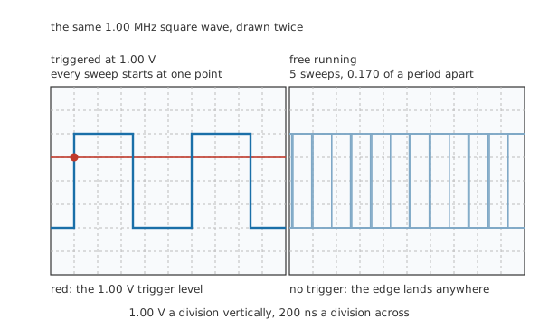
Both panels carry the same signal on the same settings. Only the moment each sweep begins differs.

Practitioner

Getting a number off the screen

A quantity comes off a scope in one of three ways. You can count squares on the graticule by eye. You can drop cursors on the feature and read the difference the instrument reports between them. Or you can let the scope compute the measurement from its captured record, which is a different thing again and usually the best of the three.

Almost every timing measurement reduces to one relationship, run in whichever direction you need it:

A working order that produces numbers you can defend later:

1. Trigger on the feature you are measuring, not on some other edge that happens to be steadier. A period read between two edges the trigger never touched inherits all the drift between them.
2. Fill the screen. A trace occupying two divisions costs several times the resolution of one occupying six, and the worked example below puts a figure on it.
3. Use cursors rather than the graticule whenever the number is going to be written down. Counting squares is for deciding whether a signal is roughly right.
4. Check what an automatic measurement is actually measuring. A frequency readout on a noisy signal counts every crossing of its threshold, noise-made ones included, and reports a confident answer far too high.
5. Take the measurement twice, on two timebases. A number that moves when the sweep speed changes is a number about the instrument.
6. Write the settings down beside the number. Timebase, coupling, probe attenuation and whether the bandwidth limit was on all change what the reading means.

That factor is not an argument for never touching the cursors. Cursors are how you measure the thing you meant rather than the thing the scope's algorithm picked, and on a waveform with several features in it that difference matters more than the last decimal place.

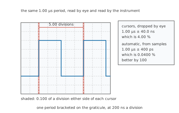
The shaded strips are the whole of the cursor reading's uncertainty. The instrument's own answer has none of it.

Engineer

The same wave, counted in frequencies

A square wave is not a different kind of object from a sine wave. It is a sum of sines: one at the signal's own frequency, the rest at whole multiples of it. For a symmetric square wave only the odd multiples survive, and harmonics works through why.

For the 1.00 MHz square wave on the screen, those land at 3.00 MHz, 5.00 MHz, 7.00 MHz and 9.00 MHz, and they carry on above that without ever quite stopping.

Each one's amplitude follows a fixed rule:

The fundamental comes out at 2.55 V — larger than the square wave's own peak, which catches everyone the first time. It is not a contradiction: the higher harmonics subtract near the middle of each flat top and add near the edges, and the sum settles at the right level. After that the amplitudes fall as one over the harmonic order, to 849 mV, 509 mV, 364 mV and 283 mV. The bars below stop at harmonic 9 — not because the series does, but because the page has to.

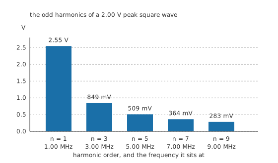
One over the harmonic order is a slow decay. The ninth is still more than a tenth of the fundamental.

What an FFT display shows instead

A scope's maths function will transform a captured record into amplitude against frequency, and the vertical axis is almost always in decibels rather than volts. Decibels covers the unit; here it does one job, which is to turn a ratio spanning a large range into a scale you can read at both ends.

Referred to the fundamental, that puts the fundamental at 0.0 dB by definition, the third at -9.5 dB, the fifth at -14.0 dB, the seventh at -16.9 dB and the ninth at -19.1 dB. Plot those against harmonic order on a logarithmic axis and they fall on a straight line whose slope is -20.0 dB for every tenfold step in harmonic order. That straight line is what a square wave looks like on an FFT display, and a departure from it is a sign that the waveform is not the symmetric square you assumed.

Most FFT displays report RMS rather than peak, which shifts every reading by the same factor:

so the fundamental appears as 1.80 V on an instrument scaled that way. The relative levels do not move, which is why a display in decibels relative to the fundamental is unaffected by the choice.

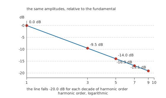
The same numbers as the bars above, on axes that turn the pattern into a straight line.

Putting the wave back together

The sum runs in both directions, and running it forwards is the most convincing demonstration that the harmonics are real rather than a bookkeeping device. Each term is an ordinary sine at its own frequency:

which gives 6.28 Mrad/s for the fundamental, and every harmonic uses a whole multiple of it in:

One term is a sine and nothing else. Three terms already have flat tops and recognisable edges. Five terms look like a square wave with a ripple beside each edge, and adding more terms narrows that ripple without shortening it, which is the behaviour Fourier series treats properly. A real square wave from a real generator has no such ripple, because its edge is finite rather than instantaneous and the series that describes it converges.

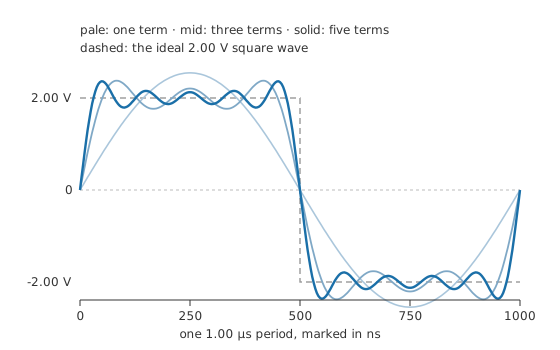
The ripple beside each edge narrows with every term added and never gets shorter.

The practical consequence sits in the next layer. If the instrument cannot pass the harmonics, it cannot draw the edge, and it will draw a slower edge instead without saying so.

Professional

What the measurement chain adds

Every stage between the circuit and the screen has a rise time of its own. For a single-pole response, that rise time follows from the bandwidth:

A 100 MHz scope therefore contributes 3.50 ns, and a 200 MHz probe contributes 1.75 ns. Neither figure has anything to do with the circuit. They are properties of the equipment on the bench, and they are present in every edge it ever draws.

Contributions like these combine in quadrature rather than by addition:

Apply it once to the probe and the scope and the measuring chain has a rise time of 3.91 ns. Apply it again against a real edge of 2.40 ns and the screen reports 4.59 ns, which is 91.3 % slow. A straight arithmetic sum of the three would have claimed 7.65 ns — worth seeing beside the right answer, because the wrong rule overstates the damage badly enough to make a usable instrument look hopeless.

The same relationship read backwards says why. That 2.40 ns edge has an equivalent bandwidth of 146 MHz, well above the scope's own, so a good part of what makes it an edge never reaches the screen. Pulse response and rise time works the single-pole case through from the network side.

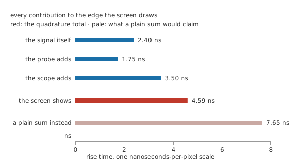
Every bar starts at the same origin on one nanoseconds-per-pixel scale. The pale bar is the answer the wrong rule gives.

Behind the arithmetic sits a first-order model, in which the front end is one pole with one time constant:

so the scope's 3.50 ns corresponds to a time constant of 1.59 ns. Real front ends are not single-pole, and a fast scope with a deliberately flat response uses a different constant in the bandwidth relationship. Instrument makers publish the figure for their own design, and an edge measurement going into a report should use theirs rather than this lesson's.

The rest of what the front panel hides

An FFT on a scope is computed from a finite record, and the record's ends are a discontinuity the transform has to cope with. The window function is how it copes, and choosing one is a trade between resolving two close frequencies and measuring the amplitude of either accurately. A rectangular window resolves best and reports amplitudes worst; the smoother windows do the reverse. A scope with the wrong window selected will show a spur that is not there, or hide one that is.

Averaging is the other setting people reach for without thinking. Several sweeps averaged together suppress noise that is not correlated with the trigger, which is most noise, and it does so at the cost of hiding anything that happens once. A glitch you are hunting for is exactly the thing averaging removes. Use it to clean up a repetitive measurement, and turn it off to go looking.

Jitter shows up as a thickening of the trace that gets worse the further from the trigger point you look, because the error accumulates over the interval between the trigger and what you are watching. Trigger close to the feature of interest and the thickening shrinks. That is also why a period measured between adjacent edges is more trustworthy than the same period measured ten cycles away.

Record length sets the outer limit on all of this, since an FFT's frequency resolution and an averaged trace's usefulness both come out of how much signal was captured in the first place. The sample-rate side of that trade belongs to using an oscilloscope.

None of these settings announces itself on the trace. A measurement written down with its settings can be checked later; one written down without them cannot, and accuracy, resolution and measurement error is where that habit gets its proper treatment. Oscilloscope probes covers the other end of the chain, which is where most of the remaining error lives.