Fourier Series: an Introduction

Intuition

Adding sines until the shape appears

A square wave and a sine wave look nothing alike on a scope. The claim behind the Fourier series is that they are close relatives anyway: take enough sine waves, at the right sizes, at frequencies that are whole-number multiples of the square wave's repetition rate, add them together, and a square wave comes out.

Start with one sine at the same rate as the square wave. It has the right timing but rounded shoulders where the square has flat tops. Add a second sine at three times that rate, sized and lined up correctly, and the shoulders flatten while the sides steepen. Add one at five times, then seven, and the flat parts get flatter while the edges get sharper. No step invents anything; each new sine only corrects what the earlier ones got wrong.

Those multiples are the harmonics of the wave, and the list of their sizes is what a spectrum analyser draws when it shows a signal as a row of vertical lines instead of a trace. The two displays hold the same information. One organises it by time, the other by frequency, and the Fourier series is the rule for moving between them.

The method came out of Joseph Fourier's work on heat conduction, long before there was any electronics to apply it to. It matters here because so much of what a circuit does depends on frequency, and a signal described as a list of frequencies is a signal you can push through a filter on paper.

Practitioner

Which frequencies, and how big

Writing a Fourier series down means answering which frequencies are allowed in the sum, and then how much of each one there is.

The frequency question has a short answer. A waveform that repeats at some rate can only contain sines that come back into step at that same rate, which restricts them to whole-number multiples of it. That multiple is the harmonic number, and anything in between would drift out of step from one cycle to the next and break the repetition:

The sizes depend on the shape, and the square wave's are the friendliest in the subject. Its even harmonics are absent altogether, and each odd harmonic's amplitude falls in proportion to its own harmonic number:

The fundamental lands somewhere unexpected: at 4/π times the square wave's peak, larger than the square wave itself. The number is right. Through the middle of each half cycle the third harmonic runs in antiphase with the fundamental and subtracts from it, pulling the sum back down onto the flat top. Harmonics approaches the same coefficients from the waveform's side, and common waveforms sets out how the other standard shapes compare.

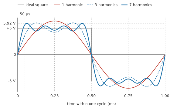
Reading the figure backwards is what makes it useful on a bench. A circuit that cannot pass the seventh harmonic of a clock hands back a rounded version of that clock, and how rounded it comes back follows from which harmonics survived the trip. Bandwidth requirements for digital signals rest on that reasoning, as does the observation that a low-pass filter in a logic path changes edges without changing levels.

Day to day the coefficients for the standard shapes get looked up instead of derived. A square wave gives odd harmonics falling as one over the harmonic number. A triangle gives odd harmonics as well, but falling as one over that number squared, so it sounds far softer. A sawtooth gives every harmonic, odd and even, falling as one over the number. Comparing a measured spectrum against the pattern you expected takes seconds, and a line where none should be is usually the more interesting finding: an even harmonic in what ought to be a symmetrical square wave says the two halves of the cycle are not matching each other, which points at an unbalanced duty or a DC offset well before anything else will.

Engineer

Averaging the waveform against each sine

Behind the square wave's tidy coefficients sits a general procedure. Any waveform that repeats can be written as a constant plus a sum of sines and cosines at every harmonic of the repetition rate. The constant is the waveform's average over one cycle, which is its DC component. Each harmonic contributes a sine term and a cosine term, and that pair collapses into a single sine of a given amplitude and a given phase shift, usually the more convenient form to carry around.

Every coefficient is found the same way. Multiply the waveform, point by point, by the particular sine or cosine you are testing for, then average the product over one whole period. Sines at different harmonics are orthogonal: multiply any two of them together, average over a period, and the result is zero. So every term except the one under test cancels itself out of the average, and what survives is that term's coefficient. The average works as a filter that keeps one harmonic and rejects every other.

Symmetry settles a good deal of it before any integrating begins. A waveform with odd symmetry, where the second half of the cycle is the first half turned upside down, has no cosine terms and no DC component. A waveform with half-wave symmetry, where each half is the negative of the half before it, has no even harmonics at all. A symmetrical square wave has both properties, so its series reduces to a bare sum of odd sine terms with no phase shifts and nothing left to work out.

With the coefficients in hand, evaluating the sum at an instant is repeated use of one relationship:

The overshoot is not a rounding error, and it does not fade as terms are added. The largest excursion of a truncated sum lands a little way past each edge, and every extra harmonic moves the peak closer to the edge without bringing it down.

The effect is known as the Gibbs phenomenon, and it belongs to the series and not to any circuit. Any calculation that truncates a spectrum inherits it, digital filters and band-limited reconstructions included.

The waveform has to repeat, at a fixed rate, without end. A single pulse that never comes back has no fundamental for anything to be a multiple of, and its proper description is the Fourier transform, whose spectrum is continuous instead of a set of lines. Data captured on an instrument is finite and sampled, so it gets the discrete version, covered further on.

At a genuine step the series converges to neither level. It converges to the midpoint of the jump, so a symmetrical square wave's series evaluates to zero at its own edges. The waveform also has to be bounded, with a finite number of maxima, minima and jumps in each period, a condition ordinary electrical signals meet comfortably.

One more limit governs what you may do with the result. Pushing the harmonics through a network one at a time and adding the outputs is valid only where the network is linear. Feed a square wave into a diode or a saturating amplifier and what comes out carries harmonics the input never had, so the list you started from no longer accounts for the answer.

Professional

What an analyser shows, and what it discards

No instrument computes a Fourier series. A spectrum display works on a finite record of samples rather than on an ideal endless waveform, so what it calculates is the discrete Fourier transform of that record, almost always through the FFT algorithm. The differences between the two account for most measurement mistakes.

A finite record has to be treated as though it repeats. If the last sample does not join smoothly onto the first, the transform sees a discontinuity that was never in the signal and smears energy across neighbouring frequencies, an effect called leakage. Multiplying the record by a window function that tapers to zero at both ends suppresses the skirts and broadens every genuine line in exchange. Picking a window is a trade between separating two close tones and spotting a small tone beside a large one.

Frequency resolution follows from the record length alone. Bins are spaced at one over the duration of the record, so resolving two components a hertz apart takes at least a second of data whatever the sample rate. Sampling faster raises the top of the range; it sharpens nothing at the bottom.

Most displays plot magnitude in decibels and throw the phase away. Two waveforms that look nothing alike on an oscilloscope can share an identical magnitude spectrum, differing only in the phase relationships between their harmonics. Where the recombined shape matters, phase has to travel with the magnitudes.

Condensing a whole spectrum into one number is what total harmonic distortion does, and the ideal square wave is a useful case to try it on.

A distortion figure means little without its conditions attached, since the result moves with level, frequency and load, and one percentage says nothing about which harmonics produced it. A low-order product and a high-order one of equal amplitude contribute identically to the total while listeners do not weigh them the same way, so audio work tends to publish a spectrum beside the number.

The same decomposition is what makes frequency-domain analysis worth the trouble. Once a signal is a list of harmonics, a linear network's effect on it reduces to a gain and a phase shift for each one, and a transfer function or a Bode plot is how that list gets written down. Interference works on the same terms: the harmonics of a fast switching edge are real currents at real frequencies, and they conduct and radiate like any other signal. EMI and EMC takes that up.