
Quick Answer
A Bode plot is a pair of graphs of a circuit's response against frequency on a logarithmic axis: gain in decibels above, phase in degrees below. Each pole bends the gain line down by twenty decibels per decade and takes ninety degrees off the phase. Straight-line asymptotes approximate both closely enough to sketch by hand.
Intuition
A response you can draw with a ruler
A filter's behaviour across frequency is a curve, and the curve is awkward to draw. The frequencies worth showing run over several factors of ten, and the amplitude at the far end may be a thousandth of the amplitude at the near end. Squeeze all of that onto ordinary graph paper and everything interesting collapses into one corner of the sheet.
Changing both axes makes the problem go away. Space the frequency axis by factors of ten instead of by equal steps, so each centimetre across the page buys another tenfold. Quote the amplitude in decibels, which does the same job going up the page. On those axes the response of a simple filter stops looking like a curve at all. It is flat on the left, a straight downward slope on the right, and a short bend joining the two near the frequency where the filter begins to bite.
That is what makes the plot worth drawing by hand. Two ruled lines and the frequency where they cross carry almost the whole answer, and the real response never wanders far from them.
Underneath the amplitude graph sits a second one on the same frequency axis, showing how far the output has slipped behind the input. A filter shrinks signals and it also delays them, by a fraction of a cycle that changes with frequency. The pair of graphs together is a Bode plot, named after Hendrik Bode, who worked on feedback amplifiers at Bell Telephone Laboratories.
Practitioner
Sketching a single pole
A pole is a frequency at which a response changes character. For the low-pass section sketched here it sits at the cutoff frequency, and two components decide where.
Worked example — Locating the pole of one RC section
A 1.6 kΩ resistor feeding a 100 nF capacitor down to ground has its pole at 994.7 Hz, within one percent of a round 1.0 kHz.
The construction below works on that round figure:
- Draw the low-frequency gain as a horizontal line and carry it to the right, as far as the pole.
- From the pole, draw a second line falling twenty decibels for every decade, meaning for every tenfold rise in frequency.
- Mark a point three decibels below where the two lines cross. The response goes through it.
- Bend the response off one line and onto the other over roughly a decade on each side.
None of that needs a calculator. What the calculator settles is how good the result is, and the gain magnitude that decides it depends only on the ratio of the frequency to the pole:
A gain is a ratio of two voltages, so the amplitude form of the decibel converts it:
Worked example — Four points against the straight lines
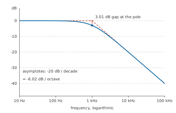
A decade below the pole, at 100 Hz, the gain is 0.995, or -0.04 dB. The flat line drawn there reads 0.0 dB, so the sketch is out by 0.04 dB.
At the pole itself the gain is 0.707 and the response is -3.01 dB, against 0.0 dB where the two lines cross. That gap is 3.01 dB.
A decade above, at 10 kHz, the gain has fallen to 0.0995, or -20.04 dB, while the sloping line reads -20.0 dB.
Another decade on, at 100 kHz, the response is 0.0100, which is -40.00 dB against a line at -40.0 dB.
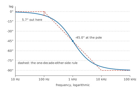
The lower graph is built the same way. Output lags input by an angle whose tangent is the ratio of frequency to pole frequency, so the lag is next to nothing far below the pole and close to a quarter cycle far above it. The rule of thumb holds the phase at zero out to a tenth of the pole frequency, runs a straight line from there down to a full quarter cycle of lag at ten times the pole frequency, and passes through half of that at the pole.
The angles themselves come out as -5.7° a decade below the pole, -45.0° at it, -84.3° a decade above and -89.4° two decades above. The rule lands on the middle figure and is at its worst at its own breakpoints, where it misses by 5.7°.
Engineer
How wrong the straight lines are
Both lines are limits of one expression, taken at the two ends of the frequency axis.
Far below the pole the squared ratio is negligible beside the one, the root goes to one, and the gain goes to unity: a horizontal line at zero decibels. Far above the pole the one is negligible beside the squared ratio, the root reduces to the ratio itself, and the gain becomes the pole frequency divided by the signal frequency.
A gain in inverse proportion to frequency loses a factor of ten in amplitude for every factor of ten in frequency, and on the amplitude scale a factor of ten is twenty decibels. Plotted against a frequency axis spaced by factors of ten, that is a straight line of constant slope. Quoted per octave, a factor of two instead of a factor of ten, the same line comes to -6.02 dB.
At the pole neither term dominates. Both are one, the root of two divides the gain, and the response is -3.01 dB while both lines still read 0.0 dB. Since one limit is only approached going down in frequency and the other only going up, the pole is where each is at its weakest, and the gap there is as far from the truth as the construction ever gets.
Worked example — An octave either side of the pole
At 500 Hz, half the pole frequency, the gain is 0.894 and the response -0.97 dB, while the flat line still reads 0.0 dB.
At 2.0 kHz, twice the pole frequency, the gain is 0.447 and the response -6.99 dB, while the sloping line has already reached -6.02 dB.
Both gaps come to 0.97 dB, the same figure on each side.
So the error is symmetric about the pole once the frequency axis is logarithmic, and it collapses quickly: three decibels at the pole, about one an octave away, and 0.04 dB a decade away. A hand sketch of a single pole is never more than three decibels wrong anywhere on the page. Without that bound the construction would be a curiosity.
The phase rule is cruder. Its breakpoints a decade either side are a convention chosen so that the line lands on the right value at the pole, and nothing forces the phase to be zero at one end of that span or a full quarter cycle at the other. The construction is exact at the pole and asymptotically right at both extremes, and worst where the convention puts its corners.
What the construction assumes
The expression describes one real pole. A zero does the opposite: it bends the slope up by twenty decibels per decade and returns a quarter cycle of phase, and the same ruler-and-pencil method covers it with the signs reversed.
A resonant network is not covered at all. Where two reactive components exchange energy, the poles come as a complex pair, and the response at the natural frequency can sit well above or well below the crossing of the asymptotes by an amount set by the circuit's Q. The three-decibel figure belongs to a single real pole and to nothing else; series RLC circuits and Q factor deal with that case.
The plot also describes a steady state. Every point on it assumes a sinusoid held long enough for the transient to die away, so the plot says nothing about the first few microseconds after a step. That view of the same single-pole circuit is the RC time constant, and the two descriptions share the same product of R and C.
Magnitude and phase are tied to each other only for a minimum-phase network, which a passive RC section is. Add a pure delay, or a zero in the right half of the complex plane, and the circuit carries extra lag that the magnitude plot gives no hint of. The magnitude alone stops being a complete description at that point, and both graphs have to be measured.
Professional
What extra poles do to the sketch
Poles add up
Cascaded stages multiply their gain magnitudes, and decibels turn multiplication into addition, so the sketches stack: slopes add, angles add.
Worked example — A second pole further up the band
Put a second pole at 20 kHz in the same signal path as the first. Two decades above the first pole, at 100 kHz, that first pole alone contributes -40.00 dB.
The second pole is only a factor of five past its own corner there, giving a gain of 0.196, or -14.15 dB. Together the pair delivers -54.15 dB, and the two lags total -168.1°.
Every pole steepens the final slope by another twenty decibels per decade and eventually costs another quarter cycle of lag. Both matter, but the phase is what turns a filter question into a stability question.
Reading the plot for stability
A feedback loop is read at one frequency in particular: the one where its loop gain passes through unity, which is zero on the decibel axis. Correction fed back with half a cycle of lag arrives in step with the error rather than against it, and a loop with that much lag at unity gain sustains its own oscillation. Two poles can only approach half a cycle; three can pass it while the gain is still above unity, so trouble tends to start where stages are cascaded inside a loop.
The gap between the lag at unity gain and half a cycle is the phase margin, quoted in degrees. A few tens of degrees is the usual requirement, with the figure set by how much overshoot and ringing the application will accept. Circuits built on negative feedback are designed against that reading.
One pole placed on purpose
Amplifier designers turn the problem round by making one pole dominate. An internal capacitor puts a single pole far below everything else, so the open-loop response is one straight slope across the whole useful range and the phase never has a chance to accumulate.
Worked example — An illustrative op-amp rolloff
Take an open-loop gain of 100 dB at DC, a voltage ratio of 100000, with a single pole at 10 Hz. These are illustrative figures chosen to show the shape, not a catalogue part.
Falling at twenty decibels per decade from there, the gain reaches unity at 1.0 MHz.
Along a slope of that shape, gain multiplied by bandwidth stays constant, which is the gain-bandwidth product on a datasheet. Closing the loop for a gain of ten leaves a tenth of the unity-gain frequency, and the closed-loop corner sits where the flat closed-loop gain meets the falling open-loop line on the plot. Real op-amp limitations works through what else moves with it.
Tolerance, and reading a measured plot
Component spread moves a pole without changing anything else about the sketch.
Worked example — Where a twenty per cent capacitor puts the pole
Keep the 1.6 kΩ resistor. With the capacitor at the top of a twenty per cent band, 120 nF, the pole sits at 829 Hz; at the bottom of the band, 80 nF, it moves to 1.24 kHz.
Those two ends are 0.176 of a decade apart on the frequency axis.
The shape is untouched, so the whole sketch slides sideways by under a fifth of a decade and keeps every slope and every gap it had. Tolerance on a Bode plot is a horizontal uncertainty, which is a friendlier thing to design around than a vertical one.
Measuring a response for real means sweeping a source across the band and recording both channels. A gain-phase analyser does it automatically; a function generator and a two-channel oscilloscope do it point by point, with the points spaced logarithmically so they land evenly across the axis. Most of what goes wrong is loading. A probe hangs its own capacitance on the node it measures and adds a pole belonging to the measurement, and a generator with real output resistance will not hold its amplitude into an impedance that moves with frequency.
Instrument conventions vary as well. Some analysers plot magnitude on a linear scale, some show group delay in place of phase, and phase is usually wrapped into a single turn, so a cascade that has accumulated more lag than that shows a jump on the trace where the circuit did nothing at all. Collecting the whole response into one expression of frequency instead of two graphs gives a transfer function, which is how active filters and band-pass designs are specified before anything is drawn.
Common mistakes
- Reading the level off the crossing of the asymptotes — the two lines meet three decibels above where the response passes. Take the crossing as the pole's location and correct the level by hand.
- Extending the sloping line back towards the pole — twenty decibels per decade is a limit reached well above the pole. An octave out it is still about a decibel optimistic, and the sketch has to bend before it gets there.
- Multiplying decibel figures for a cascade — cascaded stages multiply their gain ratios, so their decibel figures add. A product of two decibel figures means nothing.
- Trusting the phase rule as far as the magnitude rule — the straight-line phase is several degrees out at its breakpoints, and a stability margin taken off the sketch instead of the expression can flatter a loop that is not stable.
- Sketching a resonant pair as two real poles — an LC network's response at its natural frequency is set by its Q, and it can sit far above the crossing of the asymptotes. The three-decibel rule covers a single real pole only.
- Reading a wrapped phase trace as a discontinuity in the circuit — an instrument that folds phase into one turn shows a jump where nothing jumped. Unwrap the trace before counting the lag at unity gain.
Frequently asked questions
Why is the frequency axis logarithmic?
A response worth plotting usually spans several factors of ten, and on a linear axis everything below the top decade is squashed against the origin. Spacing by factors of ten gives every decade the same width. There is a second payoff: a gain falling in inverse proportion to frequency then plots as a straight line, and that is what puts the sketch within reach of a ruler.
Why does one pole give twenty decibels per decade and not some other figure?
Well above its pole, a single-pole response falls in inverse proportion to frequency, so a tenfold rise in frequency divides the amplitude by ten. On the amplitude decibel scale a factor of ten is twenty decibels. The slope is that arithmetic and nothing more, so every single real pole gives the same number.
Is a pole the same thing as a cutoff frequency?
For a single RC section the two land on the same frequency, and the words come from different places. Cutoff is a filter description, the point where the output has fallen to half power. Pole is a description of the mathematics behind the response, and it survives into circuits that are not filters at all.
Can the phase be read off the magnitude plot?
For a minimum-phase network the two are locked together, so a slope of twenty decibels per decade implies a quarter cycle of lag and a practised eye reads one from the other. A circuit containing a pure delay or a zero in the right half of the complex plane breaks that link, carrying lag the magnitude plot cannot show. Measure both when stability depends on the answer.
Who was Bode?
Hendrik Wade Bode was an engineer who worked on feedback amplifier design at Bell Telephone Laboratories during the 1930s and 1940s. The logarithmic gain-and-phase pair of graphs carries his name. The surname is Dutch in origin and is normally said as two syllables.