
Quick Answer
Q factor measures how sharply a resonant circuit responds, and bandwidth is the span between its two half-power frequencies. The two are reciprocal: bandwidth equals the centre frequency divided by Q. A high Q means a narrow passband, a large voltage or current magnification at resonance, and a long ringdown after the drive stops.
Intuition
The glass that rings and the mug that thuds
A wine glass tapped on the rim sings a clear note that hangs in the air for a second or two. A thick china mug tapped the same way gives a dull thud, over before you have registered it. Both were struck identically and both have a natural pitch. What separates them is how much of the tap's energy leaks away into heat and sound on each swing.
The glass loses very little per swing, so the note carries on for hundreds of them. It is also choosy about what will set it off. Hum a note a little away from the glass's own and it barely stirs; land on the note itself and it will start singing without being touched. The mug loses a great deal per swing, stops at once, and answers almost anything you throw at it.
Electrical resonators sit on the same scale, and the number that says where a circuit lands between glass and mug is its Q factor, or quality factor. A high Q means low loss: the ringing lasts, and the circuit is choosy about frequency. A low Q means the opposite on both counts.
The width of the slice of frequencies a resonator takes seriously has a name of its own, bandwidth, and it is simply Q read the other way up. The awkward part of the bargain is that the narrow slice and the long ring arrive together. You cannot buy one without the other. A circuit sharp enough to pick one station out of a crowded band is also slow to settle when the signal it is carrying changes.
Practitioner
Choosing a Q for the bandwidth you need
Bandwidth means the gap between the two frequencies at which the response has fallen to 0.707 of its peak value, one on each side of the centre. That level is half the power, and it is the same −3 dB point a filter's corner is defined at. Q and that gap carry the same information:
Where the centre sits is a separate question with a separate answer, settled by the two reactive components on their own:
The result arrives in radians per second, so divide by 2π for hertz.
Worked example — A specification turned into two edge frequencies
Take 100 µH and 100 pF, the pair resonance tunes with. Their natural angular frequency is 10 Mrad/s, or 1.59 MHz as an ordinary frequency.
Suppose the design calls for a Q of 50. The bandwidth that goes with it is 31.8 kHz.
Those half-power edges land at 1.58 MHz and 1.61 MHz. Outside that span the circuit has largely stopped paying attention.
Nothing so far says the circuit will oblige. Q is not a knob; it falls out of the components, and in a series loop the resistance divides:
Wire the identical three parts in parallel and the resistance multiplies instead, so the same resistor pushes Q in opposite directions depending on the topology. Everything below is the series case.
Worked example — What the coil's own loss gives instead
Suppose the only resistance in the loop is 5.0 Ω of winding loss inside the coil, with no resistor fitted at all.
Q comes out at 200, four times what was asked for, and the bandwidth at 7.96 kHz — a quarter of the width the specification wanted.
A resonator can be too sharp for its job, and this one is. Getting back to the specification means putting loss in on purpose: the loop needs 20 Ω in total, so 15 Ω of deliberate damping is added in series. Spoiling a Q is routine work and it always succeeds. Raising one past what the coil allows is the hard direction, and no amount of circuit design will do it.
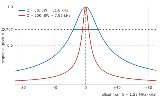
Both curves in that sweep reach the same height and sit on the same centre. Only their width differs, and the horizontal bars at the half-power level are what the bandwidth figures refer to.
Measuring a real one takes a function generator stepped slowly across the range and an oscilloscope watching the response. Find the peak first, note its height, then hunt for the two frequencies either side where the trace has dropped to 0.707 of it. Step too quickly across a sharp resonance and the peak will not have time to build to full height, which reads on the screen as a lower Q than the circuit has.
Engineer
Why the three definitions give one number
Textbooks define Q at least three ways, and a reader meeting all three inside a week is entitled to suspect they are different quantities. They are not. The definition the others descend from is about energy: Q is 2π times the energy a resonator has stored, divided by the energy it loses in one cycle. Nothing in that sentence mentions a component or a topology, so the same number describes a quartz crystal or a swinging pendulum as readily as an LC loop.
The reading that shows up on a bench is the magnification. At resonance the two reactances cancel each other in the loop, but neither has become small, and the shared current still flows through both.
Worked example — What a one-volt drive puts across the coil
Drive the low-loss loop from 1.0 V at its resonant frequency. With the reactances cancelled the winding resistance sets the current on its own, and it comes to 200 mA.
The coil's reactance has not gone anywhere. At that frequency it is 1.0 kΩ, and the same current through it develops 200 V — 200 times the source, from a generator producing a single volt.
That multiplication is worth respecting rather than admiring. Series RLC circuits treats the hazard properly, and the general practices are in electrical safety; every figure on this page came off a calculator working on a low-power tuned circuit.
Run the same circuit through the energy definition and the answer has to agree.
Worked example — The same Q counted in joules
The loop holds 4.0 µJ at the moment the coil's field is at full strength, all of it handed over by the capacitor a quarter of a cycle earlier.
One cycle lasts 628 ns, and across that time the winding resistance converts 126 nJ of it into heat.
Multiply the ratio of those two by 2π and the answer is 200, the figure the component values already gave.
The third reading, centre frequency over bandwidth, is exact for a series RLC and needs no apology. Where the two edges sit does need care. Solving for the frequencies at which the response falls to 0.707 gives a pair that straddles the centre geometrically, not arithmetically: each edge is the centre times the square root of one plus one over four Q squared, plus or minus the centre divided by twice Q.
The edges quoted in Layer 2 came out of that expression. Splitting the bandwidth evenly either side of 1.59 MHz instead misses each of them by 79.6 Hz, which is 0.25 % of the bandwidth — negligible at this Q and worth knowing about at low Q, where a wide passband and an even split can put an edge in visibly the wrong place. Multiply the two exact edges together and take the square root, though, and the answer is 1.59 MHz whatever the Q: the centre is always their geometric mean.
The time-domain reading is the same number again. Remove the drive and the ringing decays with an envelope that falls by a factor of e in 2Q divided by ω₀. For the low-loss loop that comes to 40 µs, against 10 µs for the version damped down to a Q of 50. Counted in cycles instead of seconds the answer loses its dependence on frequency altogether and becomes Q over π, so the sharp resonator rings for 63.7 cycles before its amplitude has fallen to about a third. Second-order transients works the same circuit from the step-response end, where the currency is the damping ratio and Q is one over twice it.
All of it rests on assumptions that go unstated more often than not. The parts must be linear and of fixed value: a saturating core or a voltage-dependent ceramic retunes the circuit while it is running. One frequency at a time, in steady state, with the switch-on transient already decayed — and the ringdown above is that same transient, so the two descriptions cannot both be used at once. The circuit must also be second order. Q generalises to higher-order filters as a per-section quantity, and once several sections interact, the section Q, the overall −3 dB bandwidth and the energy ratio stop being the same number. One smaller caveat belongs here too: the current in a series RLC peaks at the resonant frequency itself, while the voltage across the capacitor peaks slightly below it, by a fraction that shrinks as the square of Q. Above a Q of about ten nobody bothers with the distinction.
Professional
Loaded Q, and what the loading costs
The Q a resonator has by itself and the Q it shows once it is wired into something are different numbers, and the literature names them separately: unloaded Q for the resonator alone, loaded Q for the working circuit. Every path by which energy leaves counts against the total, and a source feeding the resonator and a load drawing from it are both such paths. Their combined contribution is written as an external Q, and the working figure is the reciprocal sum of the two, in the way conductances add.
Worked example — Unloaded, then loaded
The loop on its own reaches a Q of 200.
Connect a source and a load whose joint drain on the stored energy amounts to an external Q of 300.
The working figure falls to 120 and the passband opens out to 13.3 kHz, wider than either the unloaded resonator or the external circuit would produce alone.
Anything with an impedance that touches the resonator joins that sum, including the probe used to look at it. A design that specifies the unloaded figure and then wonders why the built filter is too wide has usually made this mistake. The usual escape is to attach the load to part of the resonator instead of across the whole of it, through a coil tap or a split capacitor, so that the load appears transformed upwards by the square of the ratio; impedance matching is the same transformation approached from the other side.
The coil almost always sets the ceiling on the unloaded figure. Its winding resistance climbs above the DC value as the frequency rises and the current crowds towards the conductor surface, the core absorbs energy of its own, and the capacitor adds its equivalent series resistance on top. All three vary with frequency, so a Q quoted without the frequency it was measured at says very little. Where the resonator is driven hard, core saturation deserves attention as well: resonance is by design the frequency at which the loop current is largest, and an inductance that collapses at peak current detunes the circuit at the moment it is working hardest.
A narrow passband makes centre-frequency stability a specification in its own right. Take an illustrative drift of one hundred parts per million, not a catalogue figure for any particular part: on this resonator that moves the centre by 159 Hz, or 2.0 % of the 7.96 kHz passband. In a wide filter such a shift would be invisible; in a sharp one the wanted signal starts sliding down the skirt. Temperature is the usual cause, ageing the slower one. Where a design needs high Q and a stable centre together, wire and dielectric struggle to supply both, and a mechanical resonator is the answer: a quartz crystal reaches a Q orders of magnitude beyond anything wound from wire, with a temperature coefficient to match.
The selectivity-against-settling trade is the constraint that bites hardest in real designs. A receiver filter tight enough to reject the neighbouring channel is also a resonator that takes many cycles to respond to a change, and a signal carrying data has to survive that smearing; pulse response and rise time treats the same limit for simple filters. Choosing Q is therefore choosing where to sit between rejecting the interferer and keeping the wanted signal intact, and the answer depends on how far away the interferer is and how fast the wanted signal moves.
Getting a trustworthy number out of a finished circuit means sweeping it, not measuring its parts one at a time. An LCR meter reports L, C and a loss figure for each component at one chosen frequency, which is useful for choosing parts and does not include the losses that only exist once everything is assembled. A swept measurement counts them all, provided the instrument's own impedance is either negligible or accounted for in the loaded figure. Q is dimensionless, so there is no unit to catch a slip; the only defence is stating the frequency and stating whether the figure is loaded or unloaded.
The same arithmetic runs through most places a tuned circuit appears. It sets the skirt steepness in band-pass and band-stop filters, decides the frequency stability and start-up time of LC oscillators, and governs how much a trap can attenuate an unwanted carrier before it starts eating the wanted one either side.
Common mistakes
- Treating a higher Q as automatically better — the sharpness and the settling time are one purchase. A filter narrow enough to reject the neighbouring signal is also slow enough to blur the one you wanted.
- Splitting the bandwidth evenly around the centre — the half-power edges straddle the centre geometrically. The centre is their geometric mean, and the even split is only a good estimate once Q is comfortably above a few.
- Designing to the unloaded Q — attach a source and a load and the working figure drops, widening the passband. Specify and measure the loaded value.
- Assuming the fitted resistor sets Q — in a high-Q loop the coil's winding resistance usually contributes more than anything on the schematic, and the capacitor's ESR is in there too.
- Quoting a Q with no frequency attached — every loss mechanism in a resonator varies with frequency, so a figure measured at one point does not carry to another.
- Reading a series expression onto a parallel circuit — resistance divides in one form and multiplies in the other, so the answer comes out wrong by a large factor with nothing about it to look suspicious.
Frequently asked questions
What does the Q factor of a circuit measure?
How much energy a resonator holds compared with how much it loses each cycle, scaled by 2π. Low loss gives a high Q. The same number also equals the centre frequency divided by the half-power bandwidth, and the factor by which the voltage or current at the reactive parts exceeds what the source supplies.
How do I work out the bandwidth from Q?
Divide the centre frequency by Q. What you get is the width of the passband between the two points at which the response has dropped to 0.707 of its peak, sitting roughly half on each side of the centre. The relationship inverts freely, so a measured centre frequency and bandwidth give you Q.
Is a high Q always what you want?
No. High Q buys selectivity and pays for it in settling time, and it also demands tighter control of the centre frequency, since a narrow passband has less room for drift. Plenty of designs deliberately add loss to widen a resonance that came out sharper than the job needs.
What is the difference between loaded and unloaded Q?
Unloaded Q counts only the resonator's own losses. Loaded Q counts those plus every path out through the source and the load, so it is always the smaller of the two and it is the one that sets the bandwidth of the working circuit. A datasheet figure for a resonator is normally the unloaded value.
Why are the two half-power frequencies not evenly spaced about the centre?
The resonant frequency is the geometric mean of the pair, not the arithmetic one, so the upper edge sits slightly further from centre than the lower. The gap between the two views closes as Q rises, and above a Q of ten or so the even split is good enough for design work.
What limits the Q of an LC circuit in practice?
The inductor, in nearly every case. Winding resistance, core loss and the coil's own self-capacitance set a ceiling that no amount of circuit arrangement can raise, and the capacitor's series resistance takes a smaller share. Reaching much beyond what a coil can offer means changing technology, to a crystal or another mechanical resonator.