
Quick Answer
An LCR meter measures inductance, capacitance and resistance by driving a part with a small alternating voltage at a chosen frequency and reading the current that comes back, in size and in timing. From those two figures it reports a value and a loss term, either as a series pair or as a parallel pair.
Intuition
The meter asks a question with a frequency in it
Ask someone a question and you learn two things from the reply: what they say, and how long they take to say it. The hesitation carries information the words do not. An LCR meter works that way. It puts a small alternating voltage across a part, measures the current that flows, and attends to both how large that current is and when in the cycle it arrives.
Size gives the magnitude of the impedance. Timing gives the phase, and phase is what separates a capacitance from an inductance from a plain resistance. A multimeter on its capacitance range does something cruder: it charges the part with a known current, times the climb, and prints a number. That is one question asked at one speed, and it says nothing about how lossy the part is.
Two parts run through this lesson. One is a 100 nF capacitor whose capacitance arrives with 0.35 Ω of series resistance, an illustrative figure for a small film part rather than a specification for any real one. The other is a 4.7 mH part whose inductance arrives with 2.8 Ω of winding resistance. Neither is a pure element, and the frequency you pick decides which half of each one you are actually looking at.
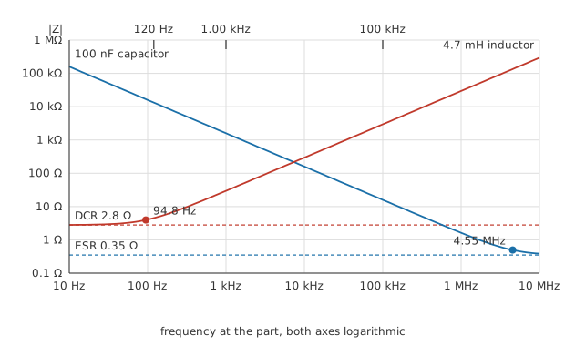
Each part is reactance over most of the span and resistance at one end of it. The two crossings, 94.8 Hz for the inductor and 4.55 MHz for the capacitor, are solved from the component values rather than read off the curves.
Practitioner
Setting the conditions before reading anything
Four settings decide what the number on the front means, and a meter that has been left on somebody else's settings will happily give you a wrong one.
- Test frequency. Standard choices are 120 Hz, 1.00 kHz and 100 kHz, and instruments with a synthesiser offer a continuous range. Pick the frequency the part will work at, or the one its supplier quoted.
- Test level. 1.00 V is a common default. A lower level keeps a non-linear dielectric or a saturating core inside its small-signal region; a higher one buys signal on a part whose impedance is awkward to resolve.
- Model. Series or parallel. Layer 3 works out why the meter asks and what changes when you answer differently.
- Fixture. Whatever holds the part is measured along with it, so the meter has open and short compensation routines to subtract it. Layer 4 shows what happens when they are skipped.
The first setting matters most, because reactance is a function of frequency and nothing else in the part is.
Those two run in opposite directions. The capacitor is 13.3 kΩ at the bottom test frequency and 15.9 Ω at the top; the inductor is 3.54 Ω at the bottom and 2.95 kΩ at the top. At 1.00 kHz they are 1.59 kΩ and 29.5 Ω, which is why a general-purpose instrument defaults there: both parts land somewhere a bridge can resolve comfortably.
Loss follows from the same arithmetic. Divide a part's series resistance by its reactance and you have its dissipation factor, written D; invert that and you have its quality factor, Q. Neither carries a unit, and neither means anything until you say at what frequency it was taken.
Worked example — The same capacitor at two ends of the range
A 100 nF capacitor with 0.35 Ω of series resistance, driven at 1.00 V.
At 1.00 kHz its reactance is 1.59 kΩ, so the test level pushes 628 µA through it. The dissipation factor is 0.00022 and its reciprocal, the quality factor, is 4547.
Move to 100 kHz and the reactance falls to 15.9 Ω. The impedance magnitude with the resistance included is 15.9 Ω, the current rises to 62.8 mA, and 22.0 mV of the applied voltage now sits across the resistance rather than the capacitance. The dissipation factor has climbed to 0.0220 and the quality factor has fallen to 45.5.
Drop to 120 Hz instead and the reactance is 13.3 kΩ, so the same test level drives only 75.4 µA. That is a small signal to resolve, and it is where a cheap instrument starts guessing.
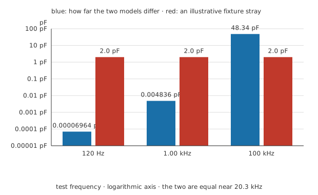
The blue bars are the subject of Layer 3. What the test frequency changes is not the part; it is how far apart the two descriptions of the part have drifted, and whether a stray you forgot to compensate still dominates them.
Engineer
One impedance, two ways to write it
A bridge measures one complex quantity per reading. Everything on the display is that quantity re-expressed, and there are two obvious ways to re-express it.
Written as a series pair, the part is a resistance with a reactance behind it, and the meter reports Cs or Ls together with Rs. Written as a parallel pair, it is a reactance with a resistance across it, and the meter reports Cp or Lp together with Rp. Both are exact. Neither is more true than the other, because a two-terminal part at one frequency has no internal structure the measurement can see.
The conversion between them runs through Q. Take the series form, add the two contributions as a complex sum and take its magnitude:
with the resistance normalised to 1 and the reactance to Q. For the capacitor at 100 kHz, where Q is 45.5, that magnitude is 45.484: barely different from Q itself, because a low-loss part is nearly all reactance. Square it and you have the factor the conversion turns on. Rp is Rs multiplied by it, and Cp is Cs divided by it and multiplied by Q².
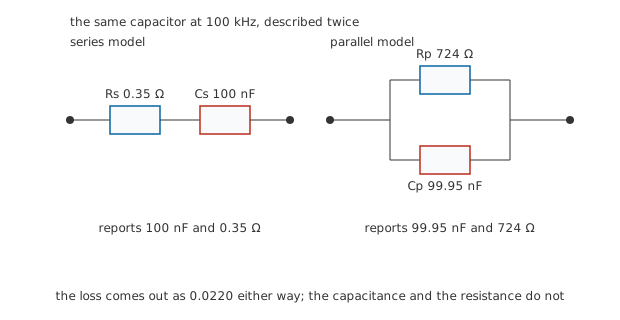
The same measurement, twice. The resistance moves by a factor of two thousand between the two descriptions; the capacitance moves by 48.3 pF.
That asymmetry is the useful part. For a good capacitor the two capacitances agree to a few parts in ten thousand, so the model barely matters if capacitance is all you want. The two resistances do not agree at all, and if you are chasing loss you have to know which one the display is showing. The working rule is to model a low impedance in series and a high impedance in parallel, because that puts the number you care about where the bridge resolves it best. A capacitor at 100 kHz is a low impedance and reads well in series; the same capacitor at 120 Hz is 13.3 kΩ and reads better in parallel.
Loss is the one figure the choice leaves alone.
At 100 kHz that is 628 krad/s, and D comes out the same whether you compute Rs divided by the series reactance or the parallel reactance divided by Rp. It has to: D is the ratio of energy lost to energy stored in a cycle, and neither of those depends on how you drew the schematic.
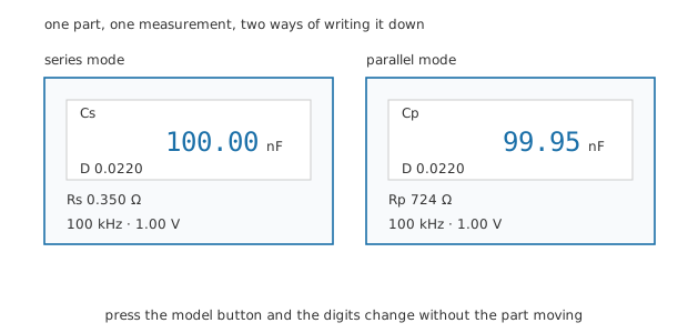
Press the model button and the two left-hand digits change while the part sits still.
Because D and Q are reciprocals, an instrument that offers both is offering one measurement under two names, and the convention is only a matter of which end of the scale a trade reads from. Capacitor people quote D, inductor people quote Q, and Q factor and bandwidth explains why the inductor trade cares more.
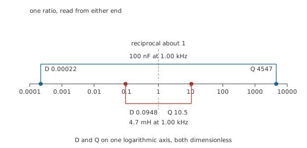
The capacitor's pair, 0.00022 and 4547, sits far out on both sides. The inductor's, 0.0948 and 10.5, sits close in, which is what 2.8 Ω of copper does to a part of this size.
The inductor is the harder case at low frequencies. At 120 Hz its reactance is only 3.54 Ω against that winding resistance, giving an impedance magnitude of 4.52 Ω and a quality factor of 1.27. More than half of what the bridge sees is copper, and the inductance is a minority share of the reading. Measure a small inductor at a frequency where its reactance dominates, or accept that you are mostly measuring wire.
Professional
What else the reading contains
A bridge reports what is between its terminals. It has no way of knowing which parts of that you meant to connect.
The fixture. Any pair of terminals has capacitance across them and inductance along them, and both are measured with the part. Open compensation records the stray with nothing fitted and subtracts it; short compensation records the series term with the terminals bridged and subtracts that.
Take an illustrative 2.0 pF of open-fixture capacitance. On the lesson's 100 nF part it is lost in the rounding. On a 100 pF part the meter reports 102 pF, an error of 2.00 %, and no amount of care with the reading recovers it. Compensation is not an optional refinement below a few nanofarads.
The leads. Every centimetre of lead adds inductance in series with the part, and at the top of the frequency range that inductance is no longer negligible against the part's own reactance.
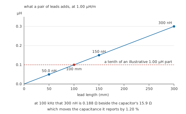
At an illustrative 1.00 µH/m, 300 mm of lead is 300 nH. Against an illustrative 1.00 µH part that is 30.0 %, and past 100 mm the leads own more than a tenth of the reading.
Against this lesson's 4.7 mH inductor the same 300 nH is 0.00638 %, which is why lead length is a small-part problem rather than a general one. It reaches the capacitor by a different route: at 100 kHz that lead inductance is 0.188 Ω of reactance in series with the capacitor's 15.9 Ω, working against it, so the meter reports a capacitance 1.20 % high. Four-terminal fixtures, which sense the voltage on their own pair of contacts, exist because the same problem shows up as resistance on low-impedance parts; current-sense resistors are measured that way for exactly that reason.
The rest of the board. In circuit, everything connected to the part's two nodes is in the measurement.
Put the lesson's capacitor at 1.00 kHz on a board where 2.20 kΩ sits across it. Described as a parallel pair the part alone is 7.24 MΩ, so the shunt swamps it and the meter now sees 2199 Ω. The Q of what it is looking at collapses to 1.38. In parallel mode the capacitance still reads 100.00 nF, because a resistance across a capacitor adds nothing to the current that leads the voltage. In series mode the same measurement reads 152 nF, with a dissipation factor of 0.724. One of those numbers is useful and the other is a fifty per cent error, and the only thing separating them is a button. In-circuit testing covers what can and cannot be done without lifting a leg.
Speed and accuracy. A cycle at 100 kHz lasts 10.0 µs, so a meter averaging over many cycles still answers quickly there; at 120 Hz the same number of cycles takes long enough that instruments offer fast, medium and slow settings and trade noise against it. The accuracy specification is a function of impedance as well as of frequency, and every instrument publishes a chart of where its best figure applies. Accuracy, resolution and measurement error sets out how to read a specification of that shape, and meter loading covers the general problem of an instrument changing what it measures.
One reading at one frequency is a single point on a curve. A part that matters gets swept, and what the sweep shows is the story the series RLC lesson tells: every capacitor becomes an inductor eventually, every inductor finds a self-resonance with its own winding capacitance, and the value printed on the part holds only below that point.
Common mistakes
- Comparing a reading against a figure taken at another frequency. A capacitance quoted at 120 Hz and one quoted at 100 kHz are answers to different questions, and for a lossy dielectric they can differ by more than the tolerance.
- Skipping open and short compensation because the part is large. It costs half a minute and it is the difference between a picofarad measurement and a guess.
- Reading Rs and Rp as though they were the same quantity. They differ by a factor of roughly Q squared, so a part described one way looks like a different component described the other.
- Measuring a part in circuit and trusting the number. Everything on those two nodes is in the reading, and the model you happen to be in decides how badly.
- Connecting a capacitor that has not been discharged. A charged part dumps into the bridge's front end, which is a repair rather than a reading, and large or high-voltage capacitors hold enough charge to be worth respecting on their own account.
Frequently asked questions
What does an LCR meter measure that a multimeter does not?
Phase. A multimeter's capacitance range times a charging ramp and reports one number; an LCR meter drives the part with a sine wave and separates the current into the part that is in phase with the voltage, which is loss, and the part that is not, which is reactance. That separation is where D, Q and ESR come from.
Which test frequency should I use?
The one the part will work at, or the one whoever specified the part used. Failing both, 1 kHz is the general-purpose default for small capacitors and inductors, 120 Hz is conventional for bulk electrolytics, and 100 kHz is where switching-supply parts are usually characterised.
Series or parallel?
Series for low impedances, parallel for high ones. The two agree closely on the reactive value for a low-loss part and disagree wildly on the resistance, so the choice matters most when the loss term is what you are after.
Is ESR the same as the Rs an LCR meter reports?
At the measurement frequency, yes: Rs is the equivalent series resistance at that frequency, and it is not a constant. It usually falls as frequency rises, then flattens, so an ESR figure without a frequency beside it is incomplete.
Why does my reading drift while I hold the part?
Body heat and hand capacitance. A hand near the fixture adds a stray of its own, and a few degrees of warming moves a ceramic dielectric measurably. Fit the part, take your hands away, then read.