
Quick Answer
Rise time is the interval an edge takes to travel from 10 % to 90 % of its final value. For a single-pole RC response it is about 2.2 time constants, and it relates to bandwidth by a constant of roughly 0.35. Every stage in a signal path adds to the rise time observed at the end of it.
Intuition
No edge is vertical
A logic gate switching from low to high is drawn on a schematic as a vertical line, and on an oscilloscope it never looks like one. The transition takes time, and the trace shows a slope with rounded corners where the voltage joins its old level and its new one.
The reason is the one that has run through this whole department. Somewhere in the path there is capacitance — in the next gate's input, in the track, in the probe — and somewhere there is resistance, in the driver's output and in the wiring. Charging that capacitance through that resistance is the same exponential approach a capacitor always makes, and the edge is just that curve seen close up.
Measuring how long the transition takes needs a convention, because the exponential technically never finishes. The universal one is to ignore the first tenth and the last tenth and time the middle: rise time is how long the signal takes to go from 10 % to 90 % of its final value. Fall time is the same measurement on the way down.
That single number turns out to be the most useful description of a fast signal there is. It sets how quickly a circuit can be clocked, how much a signal is degraded by the path it travelled, how much interference it throws off, and whether a length of wire behaves as a wire or as something more complicated. It matters considerably more than the frequency printed on the part.
Practitioner
Rise time from a time constant
For an ordinary single-pole RC response, rise time and time constant are in fixed proportion:
The factor is not an approximation of anything measured — it falls out of the exponential, as Layer 3 shows. Anything with one time constant obeys it, so the same number applies to a driver charging a load, a filter's step response, and an amplifier whose bandwidth is set by a single pole.
Worked example — A driver into a capacitive load
A driver with an output impedance of 50 Ω is charging a load of 20 pF, which is an unremarkable figure for a receiver input plus a short track.
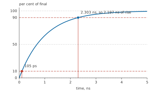
The time constant is 1.0 ns, so the edge takes 2.2 ns to get from a tenth of the way to nine tenths.
Turning that into a working limit is straightforward: a signal needs a few rise times to settle before anything samples it, so a system clocked with less than about five rise times of margin per half-cycle is already in trouble. Rise time is what actually caps clock rate, which is why a fast part driving a heavy load can be slower in circuit than a slow part driving a light one.
The three ways to make an edge faster are visible directly in the time constant. Lower the driving impedance, lower the load capacitance, or accept the edge you have. There is no fourth option in a passive path, and the first two are exactly what a buffer and a short track respectively achieve.
Fall time is worth measuring separately rather than assumed equal. Many drivers are asymmetric — a push-pull output can pull down harder than it pulls up, and an open-drain output relies on a pull-up resistor for its rising edge and so has a rise time far longer than its fall time. That asymmetry shows up as duty-cycle distortion on a square wave, growing with frequency.
Engineer
Deriving 2.2 and 0.35 instead of memorising them
Both constants are consequences of the exponential rather than empirical fits, and deriving them once removes the temptation to treat them as magic.
The response covers a fraction of the remaining distance in each time constant. Reaching 10 % takes the natural logarithm of one over nine tenths, and reaching 90 % takes the natural logarithm of ten. The rise time is the difference:
Worked example — The 2.2, from the curve itself
For the 1.0 ns time constant above, the response reaches 10 % of its final value at 105 ps and 90 % at 2.303 ns.
The difference is 2.197 ns, which is the natural logarithm of nine multiplied by the time constant. Rounded, that is the 2.2 everyone quotes.
The bandwidth constant follows from the same figure. A single-pole network's cutoff frequency is one over two pi times the time constant, so multiplying the rise time by the cutoff frequency eliminates the time constant entirely and leaves a pure number:
Worked example — And the 0.35, from the same place
The exact rise time divided by two pi times the time constant comes to 0.35.
The time constant has cancelled, so the product holds for any single-pole network whatever its component values.
Worked example — What a 100 MHz instrument can do
An oscilloscope specified at 100 MHz has a rise time of its own, of 3.5 ns, assuming it rolls off with a single pole.
That figure is not a footnote about the instrument, it is part of every measurement it makes. Cascading two single-pole stages combines their rise times as a root-sum-square rather than a plain sum:
Worked example — Measuring an edge faster than the instrument
Feed a genuine 2.0 ns edge into that oscilloscope. What appears on the screen is 4.03 ns.
The instrument has doubled the apparent rise time, and there is nothing wrong with it. Reading the trace at face value would over-estimate the edge by a factor of two.
The usual working rule follows: choose an instrument whose own rise time is around three times faster than the edge being measured, which keeps the error to a few per cent. Where that is not possible, the signal's rise time can be recovered by subtracting in quadrature — squaring the measurement, subtracting the square of the instrument's figure, and taking the root.
The conditions on all of this deserve stating. Both constants assume a single-pole response. A real amplifier or oscilloscope with a more carefully shaped roll-off has a different constant — a Gaussian response gives about 0.34, and a sharper multi-pole filter gives more, at the cost of overshoot. The root-sum-square rule likewise assumes stages that each roll off gently and do not interact. Where the response rings or overshoots, none of this applies and the circuit is not first-order at all, which is where second-order transients take over.
Professional
What rise time does to everything else
The commonest way to ruin a rise-time measurement is to make it.
Worked example — A probe that changes what it is measuring
Put a probe with 10 pF of input capacitance on a node whose driving impedance is 10 kΩ.
The probe alone gives that node a time constant of 100 ns, and therefore a rise time of 220 ns.
Whatever the node was doing before, it is now doing it a hundred times more slowly. The trace is honest about the circuit that exists while the probe is attached, and says nothing useful about the circuit without it.
That is why a times-ten probe exists: it trades signal amplitude for a much lower input capacitance, and on a high-impedance node the trade is overwhelmingly worth making. The probe's ground lead matters just as much, because its inductance resonates with the probe capacitance and puts ringing on every fast edge. A short spring-tip ground rather than a long clip lead is the difference between a usable trace and a decorative one.
Rise time, not clock frequency, is what decides a circuit's interference behaviour. The spectral content of a trapezoidal pulse extends up to roughly the reciprocal of its rise time, far beyond the clock rate, so a 10 MHz clock with a 1 ns edge radiates across hundreds of megahertz. Deliberately slowing edges that do not need to be fast — with a series resistor, a slew-rate-limited driver, or a ferrite bead — is one of the cheapest interference fixes available, and it costs nothing where the timing margin allows it.
The same number decides whether a connection is a wire or a transmission line. The comparison is between the rise time and the round-trip propagation delay along the conductor: if the edge finishes before the reflection returns, the reflection blends into the transition and nobody notices; if it does not, the trace shows steps and overshoot. That comparison, not the length alone and not the frequency, is the criterion — which is why the same track can be perfectly well behaved with one driver and a mess with a faster one.
Every stage of a real path adds its own contribution in quadrature, and the largest one dominates heavily. A path of stages at 1 ns, 1 ns and 5 ns comes out barely above the 5 ns figure, so effort spent speeding up the fast stages is wasted while the slow one remains. The technique amounts to finding the largest contributor before optimising anything.
Rise time is also a specification to read carefully rather than to compare across datasheets casually. Some parts quote 10 % to 90 %, some quote 20 % to 80 %, and logic families often quote between their own threshold voltages instead. The numbers differ substantially for the same signal, and the conditions — load capacitance, supply voltage, temperature — matter as much as the figure itself.
Common mistakes
- Reading a measured rise time as the signal's rise time — the instrument's own contribution is in there too, and it adds in quadrature.
- Comparing rise-time figures without checking the thresholds — 10-90 % and 20-80 % are different measurements of the same edge, and logic families often quote neither.
- Probing a high-impedance node with a times-one probe — its input capacitance can slow the node by orders of magnitude, and the trace then describes a circuit that only exists while the probe is attached.
- Using a long ground clip on a fast edge — its inductance rings against the probe capacitance and puts overshoot on the trace that is not in the signal.
- Assuming clock frequency governs interference — the spectrum extends to about the reciprocal of the rise time, which is usually far above the clock.
- Applying the 0.35 constant to a sharply filtered response — it holds for a single pole. Shaped multi-pole roll-offs have their own constants and their own overshoot.
Frequently asked questions
What is rise time?
The time an edge takes to travel from 10 % to 90 % of its final value. The thresholds are a convention, chosen because an exponential approach has no definite end.
Why is rise time 2.2 time constants?
Because an exponential reaches 10 % after about 0.105 time constants and 90 % after about 2.303, and the difference is the natural logarithm of nine, which is 2.197.
Where does the 0.35 in the bandwidth relationship come from?
From dividing that same 2.197 by two pi. A single-pole network's cutoff frequency is one over two pi times the time constant, so multiplying rise time by bandwidth cancels the time constant and leaves a pure number.
How fast does my oscilloscope need to be?
About three times faster than the edge you are measuring, in rise-time terms, which keeps the error to a few per cent. Slower than that and the instrument's own response dominates what you see.
Why does a slow clock still cause interference?
Because the spectral content of a pulse extends to roughly the reciprocal of its rise time, not of its repetition rate. A slow clock with fast edges radiates as though it were a much faster one.