
Quick Answer
A transfer function is the ratio of a circuit's output to its input, written as a function of frequency. Evaluating it at a frequency gives the gain and the phase there, and the values that make its denominator vanish, its poles, say how the circuit settles after a disturbance.
Intuition
What the circuit does to a signal
A steady tone fed into a filter comes back out at the same pitch, quieter than it went in and running slightly late. Change the pitch and both of those change with it. The circuit has one habit, and the habit is a rule for turning any pitch into a size and a delay.
A transfer function is that rule written down as a single piece of algebra. Hand it a frequency and it returns two numbers: how much of the input survives, and how far the output has slipped behind. Both graphs of a Bode plot are readings taken from it. So is the way the circuit settles after a switch is thrown, which those graphs do not show at all.
The word transfer is doing plain work here. The function describes what the circuit passes from its input terminals to its output terminals, and it says nothing whatever about the signal. A different signal through the same circuit meets the same rule. Separating the box from what goes through it is what makes the idea worth having, because one expression then covers every input anyone might apply to it.
That expression also turns out to be compact. Most of the circuits in this course come down to a handful of special frequencies, and once those are located the rest of the response follows from them. The special frequencies have names, poles and zeros, and a design is often finished the moment they have been put in the right places.
Practitioner
The single pole, worked through
The simplest case worth writing down is one resistor feeding one capacitor with the output taken across the capacitor, the low-pass section already met as a voltage divider whose lower leg changes with frequency. Its transfer function is the output voltage divided by the input voltage, written H, and one frequency fixes the whole of it: the cutoff, which the two components set between them.
The algebra of a transfer function is written in radians per second throughout, so the corner needs its angular form as well as its everyday one.
Worked example — A pole made out of two components
A one per cent resistor of 15.8 kΩ feeding a 10 nF capacitor puts the corner at 1007 Hz, within one per cent of the round 1.0 kHz the rest of this lesson works with.
In angular terms that corner is 6283 rad/s, and the pole of this section sits on the negative real axis at -6283 rad/s.
Written out in the frequency variable, H is one divided by the quantity one plus j times the ratio of the signal frequency to the corner frequency. The length of that quotient is the gain:
A gain is a ratio of two voltages, so the amplitude form of the decibel converts it:
Worked example — Three points on the response
Far below the corner the ratio inside the expression is negligible and the gain is 1.00: the section passes the signal untouched.
At the corner the real and imaginary parts of the denominator are equal, the root of two divides the gain, and it comes to 0.707, or -3.01 dB.
A decade above, at 10 kHz, the ratio dominates and the gain has dropped to 0.0995, which is -20.04 dB.
The same quotient carries an angle, and dividing by something with a positive imaginary part leaves the output behind the input by the arctangent of that ratio. The lag is next to nothing at the bottom of the band, one eighth of a turn at the corner, and close to a quarter turn well above it: -45.0° at the corner and -84.3° a decade above. The angles and the gains above them come from reading one expression two ways, and holding both halves of the answer in one place is the practical argument for writing a response as a ratio at all.
Confirming any of this on the bench needs a swept source and two channels: a function generator into the input, an oscilloscope across input and output together, and a note of the amplitude ratio and the time shift at each frequency. The phase reading is the fiddlier of the two and the one worth taking care over.
Engineer
Why the variable is s
The frequency has gone in so far as a real number and come back as a magnitude and an angle. The compact form replaces the whole of j times the angular frequency with one symbol, s, and writes the response as H(s). For a sinusoid held long enough for the start-up transient to die away, s is purely imaginary and equals j times the angular frequency, so the frequency response H(jω) is H(s) evaluated along the imaginary axis and nowhere else. Off that axis s carries a real part as well, written σ, and a real part describes an amplitude that is itself changing: negative σ an exponential decay, positive σ an exponential growth. The frequency response occupies one line of the plane. Everything the circuit does when nobody is driving it occupies the rest.
In s, the single-pole low-pass is one divided by the quantity one plus s over the corner angular frequency. The denominator vanishes when s equals minus that frequency, and a value of s that empties the denominator is a pole. Multiply top and bottom by the corner frequency and the same expression reads as a constant over the quantity s plus the corner frequency, which is the form to hold on to: a fixed number on top, and underneath it the gap in the plane between the pole and wherever s has been put.
Put s on the imaginary axis at some frequency and that gap becomes a length, measured from the pole to the point. Pythagoras delivers it, with the pole's own distance from the axis as one side and the frequency as the other:
Worked example — The gain read as a ratio of two lengths
At zero frequency the point of interest is the origin, and its distance from the pole is 6283 rad/s. The constant on top has that same value, so the two cancel and the gain is unity.
At the corner the point has climbed the axis to a height equal to the pole's distance from it, and the length becomes the diagonal of a square: 8886 rad/s. The gain is the constant divided by that, 0.707.
A decade higher, at an angular frequency of 62832 rad/s, the point has risen far enough that the length is barely more than the height itself, 63145 rad/s, and the gain has fallen to 0.0995.
Those two gains match the ones computed from the magnitude expression in Layer 2 to every digit published, and they had to: the length is the size of the denominator, and taking the square root of one plus a squared ratio is the same operation dressed differently.
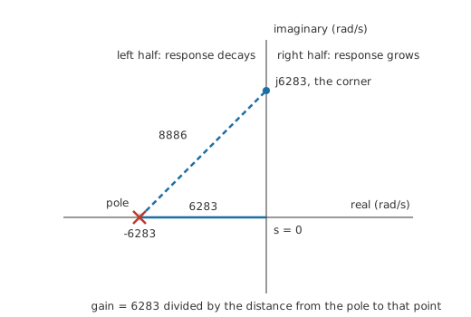
The picture extends without new machinery. A response with several poles has a length for each of them and the gain is the constant divided by the product of all those lengths, so a point on the axis that passes close to a pole sees one length shrink and the gain climb. A zero, a value of s that empties the numerator instead, contributes its length on top and pushes the gain the other way.
Nothing in the notation announces what the method assumes, so it has to be said outright. The circuit has to be linear, so that the response to a sum of inputs is the sum of the responses; a stage that clips or a junction that switches on at a threshold has no single ratio describing it. It has to be time-invariant, so the components are not changing while the measurement runs. The ratio also describes a circuit starting from rest, and charge already sitting on a capacitor when the input arrives contributes a term the ratio does not carry. One further case is a mathematical edge more than a circuit anyone builds: a pole sitting on the imaginary axis itself, with no real part at all, describes a response that neither dies nor grows. Series RLC networks put their pair of poles well off the real axis, at a height that fixes the ringing frequency and a depth that fixes how quickly the ringing stops, and second-order transients works the same pair from the time side.
Professional
Poles inside a feedback loop
Closing a loop relocates the pole
An amplifier of gain A with a network returning a fraction of its output to its input has a closed-loop response of A divided by one plus A times that fraction. The whole effect of the loop is algebra performed on a ratio, and no part of the circuit has to be redrawn to see it.
Worked example — One loop around the same pole
An amplifier has a low-frequency gain of 1000, which is 60.0 dB, and its only pole is the one already located. Returning a fraction 0.10 of the output to the input makes the loop gain 100.
The closed-loop gain is the open-loop figure divided by one plus that, giving 9.90, and the pole moves outward by the same factor, to 101 kHz.
Gain is surrendered and bandwidth recovered in the same proportion. None of this removed the pole. The pole moved, and where it moved to is the only thing in the expression that changed.
What the surrendered gain buys
Worked example — A lift in open-loop gain, and what survives of it
Raise the amplifier's open-loop gain to 1200, a change of 20.0 %, and leave the feedback network untouched. The closed-loop gain moves to 9.92, an increase of 0.165 %.
With the loop gain large, the closed-loop ratio approaches one divided by the returned fraction, and the amplifier's own gain almost drops out of the answer. A pair of resistors holds its ratio across temperature and across a production run far better than a transistor stage holds its gain, so trading most of the gain away for that stability is usually the right bargain.
A pole on the wrong side of the axis
Setting the denominator of the closed-loop expression to zero locates the closed-loop poles, and where they land is what the word stability means. Keep every one of them in the left half of the plane and every natural response decays. Let one cross over and the arithmetic reverses.
Move the pole in the figure straight across the imaginary axis, to plus 6283 rad/s, and its natural response stops decaying and starts growing, on a time constant of 159 µs and doubling every 110.3 µs. Nothing has to drive it. Circuit noise is enough of a seed, and a few milliseconds later the amplifier has left its linear region and is doing whatever the supply rails permit: a rough oscillator if the limiting is gentle, a failed part if it is not.
Poles nobody drew
The poles that decide a real design are not always the ones on the schematic. Stray capacitance across a feedback resistor, the input capacitance of the following stage, a source impedance working into a cable: each contributes a pole, usually far enough up the band to be forgotten, and the forgotten ones matter when the loop gain is still above unity where they act. Some switching-converter topologies carry a zero in the right half of the plane, which removes phase the way a pole does while lifting gain the way a zero does. No amount of loop gain cancels it, and the usual answer is to place the crossover below it.
Reading all of this off a graph instead of off the plane is Bode's construction, and the two carry the same information in different shapes: the plane is better for asking where the poles are, the graph better for asking what happens at a particular frequency. Simulators report poles and zeros directly from a small-signal analysis, and active filter design runs the other way round, starting from a wanted pole pattern and working back to component values. Choosing the pattern first is the normal order of the work.
Common mistakes
- Treating H(s) and H(jω) as two separate descriptions — the second is the first evaluated along the imaginary axis. A frequency response is one slice through the transfer function, and the transfer function holds the rest of the plane as well.
- Reading a pole as a frequency the circuit cannot pass — a pole is a value of the complex variable, and the response at the corresponding real frequency is perfectly finite. Only the algebra becomes infinite, at a point no signal generator can reach.
- Cancelling an unwanted pole with a zero on paper — the cancellation is exact only if the two land on the same point, and tolerance guarantees they will not. A right-half-plane pole hidden behind an imperfect cancellation is still there and still growing.
- Applying a transfer function to a circuit that is not linear — no single ratio describes a stage that clips or a junction with a threshold in it. A small-signal transfer function is valid only for excursions small enough to stay inside the linear patch it was taken at.
- Forgetting that the ratio assumes a circuit at rest — charge already on a capacitor when the input arrives adds a term the transfer function does not carry, and a simulated step from a settled operating point can differ from one taken from cold.
- Quoting the magnitude and dropping the angle — both come out of the same expression, and stability is decided by the angle. A response reported as gain alone cannot answer the question that most often matters.
Frequently asked questions
What is a transfer function, in one sentence?
It is the ratio of a circuit's output to its input, written as a function of the complex variable s, so that evaluating it at a frequency returns the gain and the phase shift there while the values that empty its denominator describe how the circuit settles.
What is the difference between s and jω?
The variable jω describes a sinusoid of steady amplitude, which is one line through the complex plane. The variable s covers that line and everything either side of it, its real part standing for an amplitude that decays or grows. Setting the real part to zero recovers the frequency response from the more general expression.
How many poles does a circuit have?
As many as it has independent energy-storage elements, once capacitors and inductors that can be combined have been combined. One RC section gives one pole and an RLC network gives two, so a cascade has as many as its sections carry between them.
Do I need the Laplace transform to use a transfer function?
Not to use one on a filter, where substituting jω for s and evaluating gets the answer. The transform is where the variable comes from and what justifies treating a derivative as a multiplication by s, so it matters as soon as the question moves from steady response to what happens after a step.
What makes a right-half-plane pole fatal?
A positive real part describes a natural response that grows exponentially with no input driving it. Noise inside the circuit is enough to start it, and the growth continues until the circuit leaves its linear region. Nothing added at the input can suppress it.