
Quick Answer
Resistor tolerance is the band, given as a percentage of the marked value, within which the manufacturer promises the true resistance lies at a stated reference temperature. A tighter tolerance costs more and buys a narrower band. It says nothing about how the value drifts afterwards, and nothing about where in the band any particular part sits.
Intuition
A marked size, not a measured one
Buy shoes marked size nine and you have not been told the length of the shoe. You have been told which bin it came out of. Two pairs in that size, from two makers, differ by enough to notice, and nobody files a complaint, because the marking was a band from the beginning.
A resistor works the same way. The coloured bands or the printed code name a nominal value, and one further marking names the tolerance: the width of the bin. A part marked 3.32 kΩ with a tolerance of ±1 % is a promise that its true resistance lies between 3.287 kΩ and 3.353 kΩ. Every value in that span is a good part. None of them is the marked value.
This is not a factory apologising. Holding a film element to a hundredth of a per cent is possible and expensive; holding it to five per cent is nearly free, and most of a circuit does not care which it gets. The tolerance figure is how a maker sells you exactly as much precision as you asked for. What it asks in return is that you design for the whole band rather than for the number the colour code prints on the body.
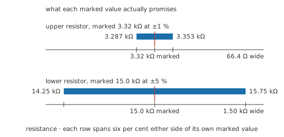
Both rows span the same fraction of their own marked value, so the looser band comes out five times the width of the tighter one.
Practitioner
Working out what the band allows
Put the tolerance in as a signed percentage and one expression gives you either end of the band.
That much is arithmetic anybody can do in their head for round numbers. The interesting part starts when two such parts have to work together, because the circuit inherits both bands at once and not always in the way you would guess.
The standard case is the voltage divider, which turns two resistances into a fraction of a supply:
Worked example — What the divider is allowed to do
An upper resistor marked 3.32 kΩ at ±1 % sits above a lower one marked 15.0 kΩ at ±5 %, fed from 3.30 V.
With both parts exactly on their markings the output is 2.7020 V. The chain draws 180 µA, which leaves 598 mV across the upper part and the rest across the lower.
The upper part is allowed anywhere from 3.287 kΩ to 3.353 kΩ, a span of 66.4 Ω, and the lower from 14.25 kΩ to 15.75 kΩ, a span of 1.50 kΩ. Four pairings, four outputs: 2.6714 V, 2.6815 V, 2.7207 V and 2.7302 V.
The two that sit furthest apart are the upper part at its high limit with the lower at its low limit, and the reverse of that. Between them the output may be 30.6 mV below the nominal figure or 28.3 mV above it, which is -1.13 % and 1.05 % in proportional terms.
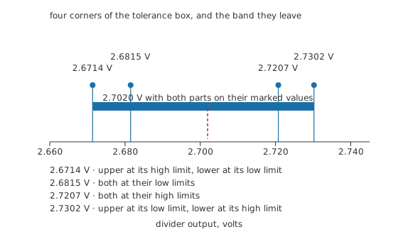
The two middle corners are the pairings where both parts err the same way, and they cost far less than the two that err oppositely.
Notice which corners hurt. Both parts high together, or both low together, barely moves the output at all — a divider cares about the ratio of the two resistances rather than about either one on its own. The damage comes from the pairings that pull in opposite directions. That is the first hint that a tolerance stack is not simply the sum of the parts, and Layer 3 makes it exact.
Engineer
Why the output moves less than the parts do
The output band above is narrower than the lower resistor's own ±5 %, and that is worth deriving rather than noticing. Write the divider as the supply divided by one plus the fraction R1/R2, and ask how much a small fractional change in either resistance moves the result. The answer, for both of them, has the magnitude R1/(R1 + R2), positive for the lower part and negative for the upper. Here that factor is 0.181.
So a one per cent error in the upper part does not produce a one per cent error at the output. It produces 0.181 %. The lower part's larger tolerance produces 0.906 %. Tolerance money belongs where the sensitivity is, and in this divider that is emphatically the lower resistor, even though the upper one is the smaller resistance.
Worked example — Guaranteed limit against statistical spread
The two contributions are 0.181 % and 0.906 %.
Assume both parts sit at their worst limits and in opposing directions, and the contributions simply add: 1.09 %. That is a guarantee, and it matches the exact corner arithmetic of Layer 2 to within the small asymmetry those corners carry, because the divider is not quite linear in either resistance.
Assume instead that the two errors are independent, and they combine as a root sum of squares: 0.924 %. The guaranteed figure is 1.18 times the statistical one.
The root-sum-of-squares combination has no entry in this site's formula library, so the number above is computed directly in the lesson's verification script rather than rendered from a stored expression. The same combination appears in accuracy, resolution and measurement error, where it stacks two instrument specifications instead of two components; the arithmetic is identical and the caveats are the same.
Those caveats deserve a paragraph, because the smaller number is the one everybody wants. A root sum of squares assumes the errors are independent draws from distributions you know something about. A reel of resistors is not that. It is one production run, whose parts may cluster anywhere inside the guaranteed band, and whose distribution the datasheet does not describe and is under no obligation to. Some processes even sort: the tightest parts are pulled out and sold at a higher grade, which can leave the remainder distributed away from the centre rather than around it. Use the quadrature figure to describe what you expect from a production population. Use the sum when a limit has to hold for every unit you ship.
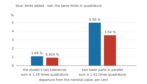
Two parts in parallel show the same split more starkly, and they also show its limit: no amount of paralleling narrows the guaranteed band.
Paralleling two parts is where this distinction gets misunderstood most often.
Two of the lower resistor in parallel come to 7.50 kΩ, and people reach for that arrangement believing it averages out the error. It averages nothing in the worst case: if both parts happen to sit at their high limit, the pair sits at its high limit too, so the guaranteed band stays at 5.00 %. What does improve is the statistical spread, which falls to 3.54 %, better than a single part by a factor of 1.41, which is the square root of two. Whether that is worth two components and two solder joints depends entirely on which of the two numbers your specification is written against.
The corner arithmetic was pointing at one more thing. Plot the two resistances against each other and the tolerances define a rectangle of pairs a buyer might legitimately receive. Every pair on a straight line through the origin gives the same output, because only the ratio matters.
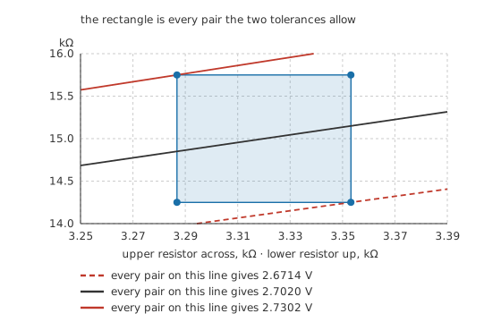
Only two corners of the rectangle touch the extreme lines. A pair that moves along a line changes both resistances and leaves the output exactly where it was.
Professional
What the tolerance figure does not cover
The band on the datasheet is a statement about the part as it leaves the factory, at a stated reference temperature, before anything has happened to it. Four things happen to it.
The first is temperature. A tolerance figure and a temperature coefficient are separate specifications and they add up.
Take the upper resistor with a coefficient of 100 ppm/°C and warm it by 50 °C. A part that started exactly on its marked value ends at 3.3366 kΩ, a shift of 0.500 %. A part that started at its upper limit ends 1.505 % above the marked value, and one that started at its lower limit is now only -0.505 % away. The band has not widened. It has travelled — by half of what the tolerance allows on either side — and a design checked only at the cold corners has missed the warm ones entirely.
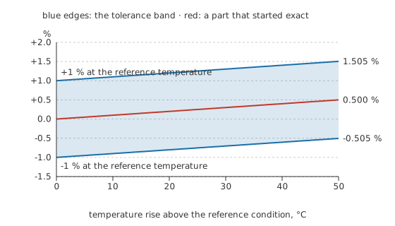
Temperature moves the whole band rather than stretching it. A coefficient with a tolerance of its own would stretch it as well.
The second is that two parts of the same tolerance do not necessarily agree with each other. Tolerance is an absolute promise about each part separately, and a divider, a bridge or a gain-setting pair cares about how well the two match. Parts from one reel usually match better than the band implies, and parts on one substrate, cut and trimmed together, match far better still and drift together as well. Matching is a separate purchase, written on its own line of the datasheet as a ratio tolerance or as a tracking coefficient in parts per million per degree.
The third is time. Resistance moves slowly under load, under humidity, after soldering and after mechanical shock, and the initial tolerance says nothing about any of it. Where it matters, a stability or load-life figure is the specification to look for.
The fourth is measurement. A band you cannot see is a band you cannot verify, and the instrument has an uncertainty of its own. Suppose the divider's output is checked with a meter specified at ±0.1 % of reading plus 2 counts, on a range whose last digit is worth 0.500 mV.
That comes to ±3.70 mV, against a band the parts may occupy running from 30.6 mV below nominal to 28.3 mV above. The band is 7.95 times as wide as the meter's uncertainty, so what the reading shows is the components rather than the instrument. Halve the tolerance twice and that comfort disappears; the general rule and its arithmetic live in accuracy, resolution and measurement error.
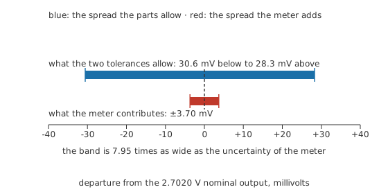
A measurement is only evidence about a tolerance when the instrument's own band is small compared with the one being checked.
Practical selection follows from all of this rather than from a preference for tight parts. Work out which resistances the output is actually sensitive to and buy precision there. Accept ±5 % where the sensitivity is low, since construction type and coefficient often matter more than the initial band. Remember that a tight tolerance is useless if the value you want is not stocked, which is what the E-series exists to settle, and that the rest of the choice is worked through in choosing the right resistor.
Common mistakes
- Designing on the nominal value and checking the extremes afterwards — the extremes are the design. Evaluate the corners first, and treat the nominal answer as the one case guaranteed not to occur exactly.
- Buying tight tolerance everywhere — precision is worth paying for only where the output is sensitive to that particular resistance. Work out the sensitivity, then spend.
- Quoting a root sum of squares as a guarantee — it describes a population, not a unit. A limit that must hold for everything you ship is the sum of the limits.
- Assuming two parts marked with the same tolerance track each other. Matching and tracking are separate specifications, and buying them means buying arrays or ratio-specified pairs.
- Reading a tolerance band with an instrument whose own uncertainty is a large fraction of it, then reporting the result as though the meter contributed nothing.
Frequently asked questions
Does a tighter tolerance mean the part is closer to its marked value?
It means the guaranteed band around the marked value is narrower. Any individual part may sit anywhere inside its band, and a loose part that happens to measure close to nominal is not thereby a tight part, because nothing prevents the next one from sitting at the edge.
Where inside the band do real parts actually sit?
The datasheet does not say, and you should not assume a bell curve centred on nominal. Manufacturing distributions vary between processes, and where a maker sorts the tightest parts out to sell at a higher grade, what remains can be distributed away from the centre.
Can I measure a batch and select the ones I want?
You can, and it is a real technique for one-off work. What you have selected is the value at the time and temperature you measured it. The temperature coefficient, the load-life stability and the ageing behaviour are untouched by your selection, so a selected loose part is not equivalent to a bought tight one.
Why do precision resistors come in values like 4.99 kΩ instead of 5 kΩ?
Because the preferred-value series is spaced logarithmically to suit a tolerance, and a tighter tolerance calls for a denser series with its own odd-looking values. The spacing is chosen so the bands of neighbouring values nearly meet without leaving gaps.
Does the tolerance apply at any temperature?
No. It is quoted at a reference condition, usually room temperature, and the temperature coefficient describes the departure from there. Both specifications have to be carried into a worst-case calculation for a circuit that runs warm.