
Quick Answer
Nodal analysis solves a circuit by choosing one node as the voltage reference, assigning an unknown voltage to every other node, and writing Kirchhoff's current law at each unknown node with every branch current expressed as a voltage difference divided by a resistance. Solving the resulting equations gives every node voltage, and every branch current follows.
Intuition
A junction sits where its currents balance
Three wires meet at a point. Two of them come back from supplies whose voltages are already known; the third runs down to the rail everything else is measured against. The junction carries no marking of its own and no one has told you what voltage it holds. It settles wherever the circuit puts it.
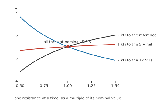
That settling point can be found by trial rather than by algebra. Pick a value for the junction, work out what current each of the three branches would carry if the junction really sat there, and see whether as much arrives as leaves.
Say the first supply is 12 V behind 2 kΩ, the second is 5 V behind 1 kΩ, and 2 kΩ runs from the junction down to the reference rail.
Test 6.0 V. The first supply pushes 3.0 mA in. The branch to the reference rail draws 3.0 mA on its own, the branch back to the second supply draws another 1.0 mA, and the two together take 4.0 mA against the 3.0 mA arriving. Charge would have to pile up at the junction at 1.0 mA, which no point in a circuit does. The trial value is wrong.
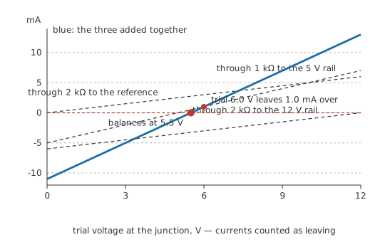
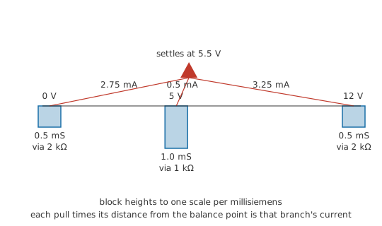
Lower it. Incoming current grows, both outgoing currents shrink, and the two sides meet at 5.5 V: 3.25 mA arrives while 0.5 mA and 2.75 mA leave, so the junction gains and loses at the same rate. Nodal analysis is that test written as an equation — one equation for each junction whose voltage you do not know — and solved rather than searched for.
Practitioner
Reference node, unknown voltages, one equation each
Start by marking the nodes. A node is a stretch of conductor at one potential: two components joined by nothing but wire share a node, however far apart the drawing puts them, and a node with four components on it is still one node.
One of them becomes the reference, and its voltage is called zero. Any node will serve, since only differences between nodes ever appear in an answer, and the ground symbol usually marks the one already chosen. Every other node gets a voltage of its own. Some of those are known before you start: a node joined to the reference through nothing but a voltage source is fixed by that source, and can be written down straight away.
What remains is one unknown per surviving node, and one equation each to match. The equation is Kirchhoff's current law — the currents leaving a node sum to zero — with each of those currents rewritten in terms of node voltages:
A resistive branch running from the node you are working at to some other node carries away the voltage at your node minus the voltage at the far one, divided by the branch resistance. Written that way, a branch current is an expression in the two node voltages at its ends rather than an unknown in its own right. A branch containing a current source is easier still, since the source states the current outright.
The library entry carries three terms, and three is also the count at each node of the circuit below. Junctions are rarely so obliging — two branches or twenty are equally possible — and a sum of unbounded width will not fit into a single expression. Kirchhoff's law is stated as a sentence for that reason, and nodal analysis leaves you with a procedure to carry out rather than an expression to fill in.
Worked example — Two unknown nodes, one of them fed by a current source
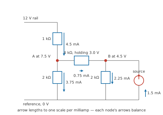
Node A hangs off a 12 V rail through 1 kΩ, with 2 kΩ of its own down to the reference rail. 4 kΩ carries on from A to node B, which has 2 kΩ to the reference and a current source pushing 1.5 mA into it. The supply holds the rail against the reference, which leaves A and B as the unknowns.
Three branches leave A. One goes to the rail, and carries A's voltage minus the rail's, over 1 kΩ. One goes to the reference, and carries A's voltage over 2 kΩ. One goes to B, and carries A's voltage minus B's, over 4 kΩ. Set the three to zero and node A's equation is written.
Node B has the same three branches to account for: the one back to A, the one to the reference through 2 kΩ, and the source, whose contribution is 1.5 mA arriving no matter what B does.
The pair solves to 7.5 V at A and 4.5 V at B.
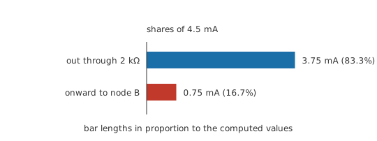
Recovering the branch currents takes a subtraction and a division each. The rail branch delivers 4.5 mA into A, and 3.75 mA of that goes straight down to the reference. Across 4 kΩ stands 3.0 V, so 0.75 mA crosses to B, joins the source's contribution, and leaves as the 2.25 mA in the last branch.
Both nodes now audit in one line. Counting everything as leaving, so that the rail branch enters negative, node A's three branches come to 0.0 mA. Node B's three, with the source likewise negative, come to 0.0 mA. That check has a definite reach: the sums come to zero by construction once the algebra is right, so a dropped term or a sign slip shows up, while a resistance entered wrongly passes it untouched.
All the unknowns in that working were node voltages, the drawing was read junction by junction throughout, and the current source went in alongside the resistors on the same footing, its contribution fixed before any equation was written. Mesh analysis has this the other way round, with current sources the awkward case there and voltage sources free.
Before any of it is written down, see whether the network collapses. Series and parallel reduction settles many circuits outright, and equations are only needed for whatever survives it.
Engineer
Writing the array straight off the connection list
The equations can also be written down whole instead of assembled a term at a time. Once every branch current is a voltage difference over a resistance, the coefficient standing in front of each node voltage is a conductance, and the connection list supplies it directly.
Put the two equations of the worked circuit side by side. On the diagonal sit 1.75 mS and 0.75 mS, each the sum of the conductances of all the branches touching that node. Off the diagonal, in both positions, sits the conductance the two nodes have in common, 0.25 mS, negated. On the right stand 12 mA, which is what the rail branch would push into A if A were held at the reference, and the source's own 1.5 mA.
In general, the entry at row k, column k is node k's self-conductance; the entry at row k, column j is the total conductance joining nodes k and j, negated; and the right-hand entry of row k is the net current driven into node k by sources. That minus sign is forced rather than chosen. A neighbour's voltage acts on node k only through the branch between them, and raising the neighbour pulls current into k, which is the opposite sense to k's own voltage pushing current out.
That array has the same shape as the one mesh analysis produces — symmetric, self-terms on the diagonal, shared terms negated off it — while meaning something transposed. There the diagonal is a sum of resistances round a loop; here it is a sum of conductances at a point. Either way the symmetry can be used to proofread: two off-diagonal entries that disagree mean something has been miscounted.
A dependent source costs you that symmetry, since its term is built from a voltage or current elsewhere in the circuit and lands in one row with nothing to match it in the other. The array also takes a constant conductance from every branch, which is a linearity requirement, and a diode has none to give. A circuit holding one is linearised about an operating point before any of this applies to it.
A voltage source floating between two nodes
An ideal voltage source holds the difference between its terminals fixed and takes whatever current the surrounding circuit calls for. That current is whatever the rest of the network makes it, so the branch has no expression in node voltages to offer, and neither of the nodes it joins can be given an ordinary equation.
What to do about it turns on the source's position. With one end on the reference it simply fixes the other node, which stops being unknown. Floating between two unknown nodes it fixes only their difference, and the pair is treated as one region — a supernode — with current balance written round the whole region so that the source's branch never appears. The source's own statement supplies the second equation.
It is still current balance being applied, now round a boundary that encloses a region instead of a point. Three branches cross the boundary drawn below, so the same three-term sum does the work:
Worked example — A supernode across a floating source
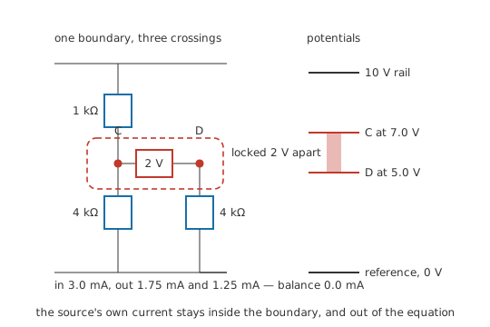
The circuit, as an inventory: 1 kΩ from a 10 V rail down to node C; 4 kΩ from C to the reference; a source of 2 V from C across to node D, positive terminal at C; 4 kΩ from D to the reference.
Draw a boundary enclosing C, D and the source. Three branches cross it: the one to the rail through 1 kΩ, the one to the reference through 4 kΩ, and the one to the reference through 4 kΩ. Balance those three. The source's own current lies wholly inside the boundary, which keeps it out of the equation altogether.
The constraint can be read straight off the drawing: C stands 2 V above D. Substituting it leaves one equation in one unknown, and the region solves at 7.0 V for C and 5.0 V for D.
The rail branch then carries 3.0 mA in, while 1.75 mA and 1.25 mA leave, so the boundary balances at 0.0 mA. The source's own current is read off last, from the node equation that could not be written: D has only the source and one resistor on it, so the source must be delivering the 1.25 mA that resistor carries away.
Circuits with no windows at all
A node is a feature of what is connected to what, and it survives any rearrangement of the page. Nodal analysis therefore places no condition on how a schematic is drawn. Mesh analysis places one, since a mesh is a window of the drawing and stays undefined until the circuit is laid out with nothing crossing; a set of five nodes with a branch between every pair cannot be laid out that way at all. Such a circuit has no windows and no mesh equations, and is entirely ordinary to analyse node by node.
A connected network of N nodes yields N − 1 independent current equations, one for each node but the reference, whose own equation is just the sum of all the others. Mesh analysis yields B − N + 1 for a network of B branches, so the two disagree about how much work a given circuit is, and that comparison is taken up further down the page.
Professional
From paper method to production solver
The unknowns a solver adds
SPICE and everything descended from it solves circuits by nodal analysis, in an extended form called modified nodal analysis. The extension exists for the case the supernode was invented to work around. An element can be stamped into the conductance array only if its current can be written as a function of the node voltages at its ends, and an ideal voltage source cannot: its current is set by everything around it.
Rather than routing round such elements with supernodes, modified nodal analysis promotes each one's branch current to an unknown of its own, and the array gains a row and a column for it, filled with entries of plus and minus one that state the source's terminal-voltage constraint. Inductors get the same treatment, and controlled sources are stamped directly, their gain terms landing in whichever rows and columns the controlling nodes occupy. The array then holds more than conductances and loses its symmetry, and in exchange the method handles any element a netlist can name.
Software favours this because each element stamps itself independently, from its own value and the node numbers it was given. A netlist is read once, element by element, in any order. Nonlinear devices are linearised at the current guess and the whole array is rebuilt each Newton iteration; capacitors and inductors become resistances and sources at each timestep. Mesh analysis offers no comparable entry point, since its windows have to be identified up front and sometimes do not exist at all.
Node count sets the bill
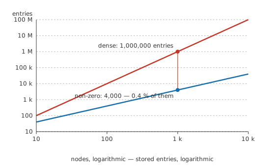
The cost of a simulation tracks the number of nodes, because that is very nearly the size of the array. Elimination on a dense array of N unknowns costs on the order of N cubed operations, which would be hopeless for anything real: two thousand nodes is a small chip.
Circuit arrays escape that because they are sparse. A node's row holds an entry only for itself and for the nodes it shares a branch with, and components have two or three terminals apiece. Give a netlist a thousand nodes with an average of three branches at each, and every row carries four non-zero entries out of a thousand: 0.4 % of the stored array holds information and the rest is zero. Sparse solvers store and factorise only the non-zero entries, and the ordering they choose for elimination decides how much fill-in — new non-zeros created by the elimination itself — they have to pay for. A large simulation's time goes into that ordering more than into the raw node count. Splitting one node in two by inserting a wire model therefore carries a cost: it enlarges the array and can spoil an ordering that was working.
Choosing where zero goes
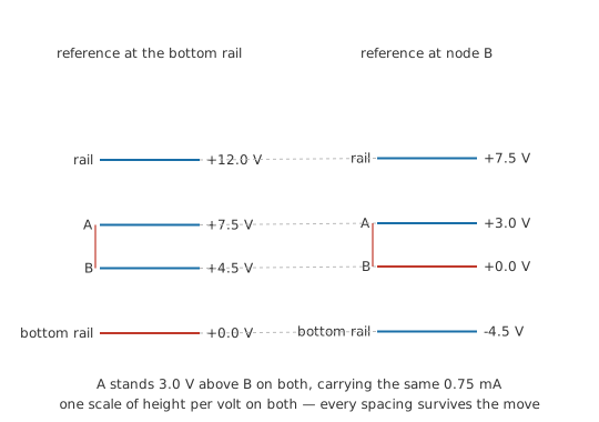
Every node voltage in a solution is measured against the reference, so moving the reference moves all of them together. Take node B of the worked circuit as the reference instead of the bottom rail. Node A comes out at 3.0 V, the old reference node at -4.5 V, and everything else drops by the same 4.5 V. Every physical quantity stands where it stood: the branch joining A and B still has 3.0 V across it and still carries 0.75 mA, and a meter clipped anywhere in the circuit reads what it read before.
Since no answer depends on the choice, it may as well be made to shorten the arithmetic. The node where the most voltage sources return is the one to pick, because each source with a terminal on the reference hands you a known node voltage for free and saves a supernode. Take node A of the worked circuit as the reference and there are three unknown node voltages instead of two, with the 12 V supply now floating between two of them and a supernode needed to cope. The circuit and its answers are the same, and the arithmetic is longer.
On a real board the choice is usually already made, and made for other reasons: the reference is the ground plane, the node a meter's black lead sits on all afternoon, and the node against which every data sheet specifies its part, so the analysis takes it as given.
Common mistakes
- Writing a branch current with only one node voltage in it. A branch between two unknown nodes carries the difference; using just the node you are standing at drops the coupling and leaves two circuits that do not know about each other.
- Sign drift between one branch and the next. Decide once that every current is counted as leaving the node, then write every term that way, including the ones you can see are physically arriving. The negative results take care of themselves.
- "Every node needs an equation." The reference does not — its equation is the sum of all the others and adds nothing — and neither does a node the sources fix outright.
- Treating a wire as a branch. A short between two points makes them one node, not two nodes with a small resistance between them. Merge them before counting; an unmerged pair produces a singular array.
- Trying to write an ordinary equation at a node with a floating voltage source on it. That branch has no current expression to write. Draw a boundary round both nodes and the source, balance the branches that cross the boundary, and take the second equation from the source itself.
- Reaching for the method before trying to reduce. Many circuits collapse by series and parallel steps into something with one unknown or none at all. Save the equations for whatever survives that reduction.
Frequently asked questions
Which is less work, nodal or mesh analysis?
Count before choosing. Nodal analysis produces one equation per node bar the reference; mesh analysis produces one per window of the drawing. Circuits with few nodes and a crowd of components between them favour nodal. A long chain of stages, with a node at every junction and few windows, goes the other way. The sources tilt it further — current sources are free in a node equation, voltage sources are free in a loop equation — and if the drawing cannot be laid flat, nodal analysis is the only one of the two available.
Does the reference node have to be the circuit's ground?
No. The mathematics treats every node alike, and any of them can be called zero. Choosing the ground node is a convenience: it is where most voltage sources return, so it makes the most node voltages known outright, and it matches how measurements and data sheets are quoted.
What happens if I get a negative node voltage?
It means that node sits below whichever node you called zero, which is ordinary. Leave the drawing and the equations exactly as they are; the branch currents computed from it come out with the right signs on their own.
Can nodal analysis handle AC circuits?
Yes. Conductances become admittances, the source values become phasors, and the arithmetic turns complex. The array is built exactly as before, with self-admittances down the diagonal and shared admittances negated off it. Which points count as nodes is unaffected by capacitors and inductors.
Why does my array come out singular?
Usually a plain wire joining two nodes has gone into the netlist as two separate nodes, or part of the circuit has no conductive path to the reference at all — a section coupled only through capacitors, say, which at DC is floating. Solvers report that second case as a node with no DC path to ground and refuse to continue.