
Quick Answer
AC circuit analysis solves a sinusoidal circuit by converting every component to an impedance at the working frequency, then applying the same network theorems used on DC circuits. Ohm's law, Kirchhoff's laws, nodal and mesh analysis and Thévenin equivalents all carry over, provided each voltage and current keeps its phase angle.
Intuition
Same laws, one extra number
A resistor network yields to rules learned early on: what arrives at a junction leaves it, the voltage drops round any loop cancel, and each resistor's voltage is its current multiplied by its resistance. Add a capacitor and drive the circuit from a source that reverses many times a second, and not one of those rules fails. What changes is the kind of number each rule is applied to.
Put a resistor and a capacitor in series across a 10.0 V source and read each drop with a meter. The resistor shows 8.102 V and the capacitor 5.861 V. Add them and the loop shows nearly fourteen volts of drop while the source supplies ten. Both readings are honest and the loop rule is intact. The two drops never reach their peaks at the same instant, so the sum a meter invites you to take counts voltage that is never present all at once.
Every signal in the circuit is still a sine wave at the source's frequency, and one such wave differs from another in only two respects: how tall it is, and how far along the cycle its peak falls. Carry both figures instead of one and the old rules go back to working as they always did. Opposition in ohms becomes impedance, which has a size and a timing. Each voltage and each current gains a timing to match, and the arithmetic that joins them tracks the size and the timing together.
Practitioner
One frequency, then solve it like DC
The procedure has a fixed order, and most of the trouble people have with it comes from taking the steps out of that order, not from the arithmetic inside them.
Fix the frequency before anything else. Until it is written down, a capacitor's opposition and a coil's opposition have no value at all.
Each capacitor becomes that many ohms, each inductor becomes its inductive reactance at the same frequency, and each resistor stays what it was. The circuit is now a network of ohms with a quarter-cycle marker attached to every reactive one.
Combine those ohms as the topology dictates, remembering that a resistance and a reactance meet at a right angle instead of end to end:
Then solve. Ohm's law accepts an impedance in the slot the resistance used to occupy, and hands back magnitudes belonging to the one frequency fixed at the start:
Worked example — A resistor and a capacitor in series, worked end to end
A source of 10.0 V RMS at 1.0 kHz drives 1.0 kΩ in series with 220 nF.
At that frequency the capacitor is worth 723.4 Ω of reactance. Stood against the resistance at a right angle, the pair presents a magnitude of 1234 Ω at an angle of -35.88°, negative because the only reactance in the chain is capacitive.
The source voltage over that magnitude leaves 8.10 mA, and a series chain shares its current, so that figure belongs to every part of the loop.
The resistor turns it into 8.102 V and the capacitor into 5.861 V. The angle says the current reaches its peak first and the source voltage arrives behind it.
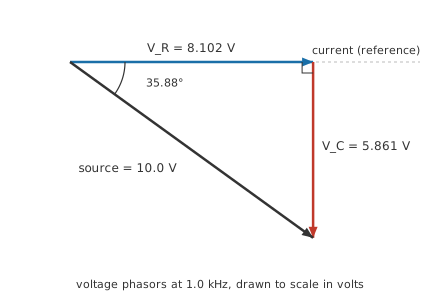
The drawing takes the shared current as its reference direction and places each voltage where its peak falls against that. The resistor's drop lies along the current because a resistor does not delay anything. The capacitor's hangs a quarter cycle behind. Laid head to tail they close on the source, and the closing side is ten volts long however carefully the other two are measured.
Everything the calculation produced belongs to 1.0 kHz and to nowhere else on the axis, so write the frequency beside the answer. Convert prefixes to plain ohms, farads, henries and hertz before anything is squared, since a nanofarad entered as a microfarad still returns a plausible-looking number. And if the chain holds a coil as well, the two reactances go in with opposite signs and partly cancel before the right triangle is drawn.
Engineer
Why the DC theorems survive
Kirchhoff's two laws are statements about an instant. The current law says charge does not pile up at a junction, which is as true one microsecond into a cycle as at any other moment; the voltage law says a round trip through a loop returns to where it started. Neither has a frequency anywhere in it, so neither notices that the source is alternating. A meter reading, though, is a magnitude with the timing stripped off, and magnitudes are not the quantities either law adds up.
The step that makes the DC machinery reusable is closure. In a linear circuit driven at one frequency, once any switch-on transient has died away, every voltage and every current is a sinusoid of that same frequency. Add two of them and the result is a sinusoid of that frequency; scale one and it stays one. Differentiate one, which is what a capacitor's current and an inductor's voltage demand, and out comes a sinusoid of that frequency again, larger by the factor ω = 2πf and moved a quarter cycle along. The family is closed under everything the circuit equations do to it.
Closure is what lets two numbers stand in for a whole waveform. A phasor carries the amplitude and the phase, and complex numbers supply the arithmetic for such pairs. In that arithmetic the capacitor's differentiation becomes multiplication by a complex constant, and so does the inductor's. Every element in the circuit then obeys one relation: its voltage is its current times an impedance.
Ohm's law is that relation with a real constant. The node and loop equations of a DC circuit are assembled out of nothing but that relation and the two Kirchhoff laws, so the AC equations come out with the same algebraic shape and Z standing where R stood. Any theorem reached from that shape by algebra alone transfers untouched: nodal analysis, mesh analysis, superposition, and the Thévenin and Norton equivalents. None of them was ever a fact about resistors; each followed from linearity.
Worked example — The loop rule, audited two ways
Take the current in the worked chain as the reference. The resistor's voltage lies along it and the capacitor's hangs a quarter cycle behind, which puts the two at a right angle.
Added as plain numbers they come to 13.96 V, well past the 10.0 V the source supplies.
Treated as the two sides of a rectangle they come to 10.0 V, and the loop closes to the last digit shown.
Losing the angle costs more than that one sum. The resistive voltage divider does carry over to AC, in the sense that the output is the source multiplied by one impedance over the total, but the division has to happen on complex quantities.
Worked example — The divider with the angles thrown away
Put the reactance into the divider expression as though it were a second resistance, and the capacitor's share comes out at 4.198 V.
Its true share is 5.861 V, because the reactance is divided by the impedance magnitude of 1234 Ω, which is smaller than the arithmetic sum of the two oppositions.
The method rests on conditions the worked chain met without being asked. One frequency: a source carrying harmonics presents a different impedance to each component of itself, and no single figure covers the lot. Linear parts: a saturating core, a rectifier or an amplifier driven into clipping changes the shape of the waveform, and a signal that is no longer a sinusoid has no phasor to draw. Steady state: for the first few cycles after a switch closes the circuit belongs to first-order transients, where an impedance says nothing useful. Each condition has a standard way round it, and the multi-frequency case is taken up further down the page.
Professional
Admittances, solvers and mixed frequencies
Parts in parallel share a voltage instead of a current, so their impedances do not add. Their reciprocals do. The reciprocal of an impedance is common enough in this work to have its own name, admittance, with conductance and susceptance as its two parts. A nodal solution in AC is written in admittances for that reason: the self term at a node is the sum of the admittances touching it, just as the DC version summed conductances.
Worked example — The same answer from a node equation
The junction between the resistor and the capacitor has two branches on it. The resistor contributes 1.000 mS and the capacitor 1.382 mS a quarter turn away from it, so the self term at that node has a magnitude of 1.706 mS.
The source drives current in through the resistor's branch alone. What it pushes in, over that self term, leaves 5.861 V at the node.
Layer 2 reached the same capacitor voltage by working along the series chain. The node equation never mentions a chain at all.
Which form to work in is a matter of convenience. Rectangular components add and subtract cleanly, so series impedances and node sums are done there; polar form multiplies and divides cleanly, so ratios and Ohm's-law steps are done there. Converting back and forth mid-calculation is ordinary, and a calculator with a complex mode removes most of the tedium.
SPICE and everything descended from it works this way. An AC analysis finds the DC operating point first, linearises every nonlinear device about that point, replaces each capacitor and inductor with its admittance at the frequency under examination, and solves one complex nodal array per frequency point. One consequence follows immediately from that description: an AC sweep cannot show clipping, slew limiting or distortion of any kind, because the linearisation removed all of it before the sweep began. A circuit that looks immaculate across a sweep may still be unusable, and a transient run is what catches it.
The one-frequency condition is the one a real signal breaks most often, and superposition is the way through. Solve the circuit once at each frequency the source contains, then put the answers back together in the time domain. RMS figures at different frequencies combine in quadrature, since the cross term between two different frequencies averages to zero over a cycle.
Worked example — A steady level riding under the sine
Leave the chain alone and add 5.0 V of DC offset to the same source.
At zero frequency the capacitor is an open circuit, no current flows, and the whole offset appears across it. At 1.0 kHz the capacitor's share is the 5.861 V already worked out.
The two contributions together put 7.704 V RMS across the capacitor. Solving at either frequency on its own understates what the part sees.
The practical failures are rarely in the complex arithmetic. An answer written down with no frequency beside it is the commonest of them, and a week later it is unrecoverable. Next is a source impedance left out of the model: a signal generator with fifty ohms of its own output resistance is part of the network being solved, and so is a scope probe's capacitance across the node it is watching. Beyond that the components stop matching their symbols as the frequency climbs, since a capacitor acquires series inductance and a coil acquires self-capacitance, and series RLC circuits shows how far a small unintended reactance can move an answer.
Common mistakes
- Adding element voltages arithmetically — the drops in a series AC chain peak at different moments, so their plain sum runs high and can exceed the source. Combine them as perpendicular components.
- Dropping a reactance into a resistive formula — divider ratios, parallel shortcuts and the rest hold on AC only once the arithmetic is done on complex impedances. A reactance treated as a second resistance gives a confidently wrong answer.
- Solving without recording the frequency. Every reactance, every impedance and every angle in the result belongs to one point on the axis, and an unlabelled answer cannot be reused or checked.
- Carrying one impedance through a multi-frequency signal — a square wave, a signal with a DC offset, anything with harmonics: solve once per frequency and combine afterwards.
- Taking a clean AC sweep as proof the circuit works. The simulator linearised everything before it started, so clipping and slew limits never appear in the result; run a transient analysis as well.
- Losing the sign of the angle — the magnitude reads the same whether a network leans capacitive or inductive, and only the sign says which. A correction fitted on the strength of the magnitude alone can push the wrong way.
Frequently asked questions
Do Kirchhoff's laws still apply to AC circuits?
Yes, unaltered. Both are statements about a single instant, and they hold at every instant of a cycle. What fails is adding meter readings, which are magnitudes with the timing discarded. Add the phasors instead and both laws balance.
Does Ohm's law work on AC?
In the generalised form, yes: the voltage across a two-terminal network equals the current through it multiplied by its impedance. Working in magnitudes alone gives the right size of answer at one frequency but says nothing about timing, so the angle has to travel with it wherever power or a phase relationship is at stake.
Is nodal or mesh analysis better for an AC circuit?
The same count decides it as in DC. One equation per node bar the reference against one per window of the drawing, with current sources free in the node equations and voltage sources free in the loop equations. Turning conductances into admittances changes the entries in the array, not its size or its shape.
Can I analyse a square wave this way?
Only one harmonic at a time. Break the wave into its sinusoidal components, solve the circuit at each of their frequencies, and reassemble the output waveform from the results. A single impedance figure describes the circuit's response to one frequency and no more.
Why do the element voltages add up to more than my supply?
They peak at different moments, so a running total of magnitudes counts opposition that is never present at once. Sum them as perpendicular components and the total comes back to the supply voltage. This is normal in any circuit holding both resistance and reactance, and it becomes extreme near resonance.