
Quick Answer
Thévenin's theorem states that any linear two-terminal network, however many sources and resistances it contains, behaves at those terminals like a single voltage source in series with a single resistance. The source is the open-circuit terminal voltage, and the resistance is the one you find by looking back into those terminals with every independent source deactivated.
Intuition
Replacing a whole network with two components
The theorem makes a claim strong enough that most people meet it with some doubt. Take any arrangement of batteries, supplies and resistors — twenty parts or fifty, it makes no difference — and bring two of its points out to a pair of terminals. Connect anything you like across those terminals. Whatever happens there could have been produced by a network of two components: one battery and one resistor in series.
The correspondence is exact. The two-component stand-in delivers the same terminal voltage and the same terminal current as the original for every load you might attach, so long as the parts inside behave linearly, which resistors and ordinary supplies do.
A meter at the terminals is enough to produce both figures. Read them with nothing connected and they stand at 3.0 V. Hang 2.0 kΩ across them and the reading drops to 1.5 V, with 0.75 mA now leaving the terminals. The reading fell because something inside took up the difference, and whatever that something is built from, it behaves as a resistance of 2.0 kΩ.
From outside, those two figures are the network. Predict the next load before connecting it: 1.0 kΩ across a source of 3.0 V behind 2.0 kΩ should sit at 1.0 V and take 1.0 mA. Connect it, and it does.
The result is named after Léon Charles Thévenin, a French telegraph engineer. Its practical value is that a supply, a sensor or one stage of a circuit can be handed over as two numbers, with the schematic kept private.
Practitioner
Finding the two numbers from the circuit
When the network is drawn in front of you, both figures come out of the component values instead of a meter.
Remove the load first. The equivalent describes the network without whatever is going to be connected to it, so the load comes off before anything is calculated and goes back on at the end.
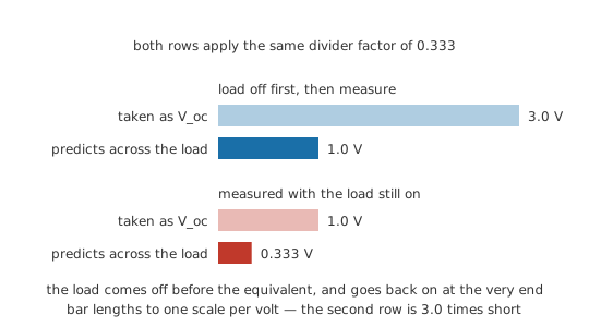
With the terminals open, no current leaves them, and the voltage that appears across them is the equivalent source value. For a two-resistor tap that is the unloaded divider result:
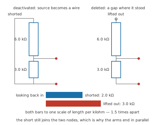
The resistance comes next. Deactivate every independent source — an ideal voltage source becomes a short circuit, an ideal current source becomes an open circuit — and work out what resistance the terminals see looking back in. Deactivating the supply of a tap puts its two arms side by side:
A single loop is left: equivalent source, equivalent resistance and load in series, with one current through all three.
Worked example — A loaded divider, worked twice
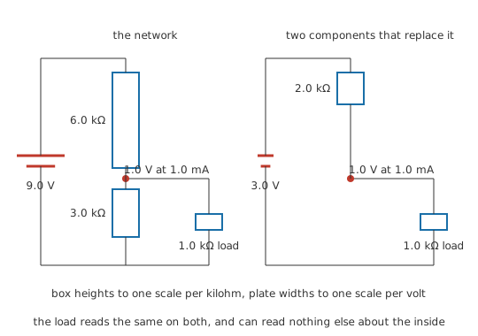
The network is a supply of 9.0 V across 6.0 kΩ above 3.0 kΩ, with the terminals taken at the junction and the bottom rail. A load of 1.0 kΩ is to be connected to them.
Open circuit, the two arms carry one current and share the supply between them, putting 3.0 V at the terminals. Deactivate the supply and its two ends become one point, which places the arms in parallel between the terminals: 2.0 kΩ. Those are the two figures the meter produced earlier, with no knowledge of what was inside.
Fit the load to the equivalent. The single loop carries I = V ⁄ (R + R_L) = 1.0 mA, and the load holds 1.0 V.
The same question can be put without the theorem at all. With the load fitted, it and the lower arm share both of their nodes, combining to 750 Ω; adding the upper arm gives 6.75 kΩ across the supply, which therefore delivers 1.33 mA. That current through the combination leaves 1.0 V at the terminals and 1.0 mA in the load. The two routes agree, as they must.
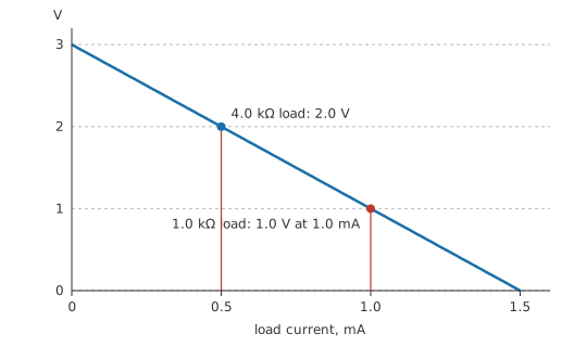
Change the load to 4.0 kΩ and the difference between the routes shows. The equivalent answers in one line — 2.0 V and 0.5 mA — while the direct route starts again from a new parallel combination, a new total, a new supply current and a new division.
The advantage shows on a network that will face several different loads, or one load whose value has not been decided. Bias networks, sensor bridges, a regulator output and the tap of a voltage divider are each characterised once and then reused. The equivalent also turns loading into a single comparison: set the load beside the equivalent resistance and the error follows from that ratio alone, which is the calculation behind a meter disturbing a high-value node.
Where the circuit is real and its schematic is not to hand, the same pair comes from measurement, and the bench procedure for getting it without damaging anything comes at the end of this lesson.
Series and parallel reduction reaches the open-circuit voltage on many circuits and on plenty it does not. A bridge, or any network the reduction cannot collapse, needs nodal or mesh equations first, and the theorem is then applied to what those give. The load is a different matter, and it may be as nonlinear as you please — a diode or a filament lamp included — since the linearity condition falls on the network rather than on whatever is hung across it.
Engineer
The straight line at the terminals
Plot what the network does at its terminals — voltage on one axis, the current leaving them on the other — and for a linear network the result is a straight line. The worked network hands you two points on it. With the terminals open no current leaves, and they sit at 3.0 V; loaded to 1.0 mA, they sit at 1.0 V. The slope between those points is 2.0 kΩ, and continuing the line to zero volts puts the short-circuit current at 1.5 mA.
A straight line has exactly two parameters: an intercept, which here is the open-circuit voltage, and a slope, which here is a resistance. Read as geometry, the theorem says that a line is all a linear network can present at two terminals, and two numbers are enough to describe a line.
Superposition supplies the proof
Why that line is straight, and why its slope is the deactivated network's resistance, both follow from linearity. In a network of linear elements, every voltage and every current is a weighted sum of the independent source values, with the weights fixed by the resistances alone. Superposition is the working form of that statement: solve for one independent source at a time with the rest deactivated, then add.
Apply it with the load replaced by a current source drawing I out of the terminals. That external source counts as one of the independent sources, so the terminal voltage is a sum of two contributions. Set I to zero — the source open, the terminals open — and the internal sources give the open-circuit voltage. Deactivate the internal sources instead, and I flows into a dead network, producing I times that network's resistance, opposing the first. Add the two and V = V_oc − I × R_th, which is a source of V_oc in series with R_th written as an equation. Two coefficients are all of the interior that survives into it.
Taken the other way round, that equation is the recipe worked through above, and the deactivation step arrives with its justification attached: it is superposition's own rule applied to the network's sources while the load's contribution is held apart.
What deactivating a source means
Setting a source to zero leaves an element behind where it stood. A zero-valued voltage source holds zero volts across itself whatever current passes through it, which is a piece of wire; a zero-valued current source passes zero amperes whatever voltage stands across it, which is a gap. That distinction does real work. Shorting the worked network's supply leaves its two nodes joined, and the joining is what brings the two arms into parallel. Lift the source out of the circuit instead and the upper arm dangles from a broken end, which is a different circuit with a different answer.
Dependent sources stay active
A dependent source takes its value from a voltage or a current somewhere inside, which makes it part of the circuit's own description rather than an input to it. Zeroing it deletes one of the equations that define the circuit, so it cannot be set to zero with everything else left intact. Superposition asks for no such thing in any case: the sum runs over the independent sources, and a dependent source stays active in every term of it.
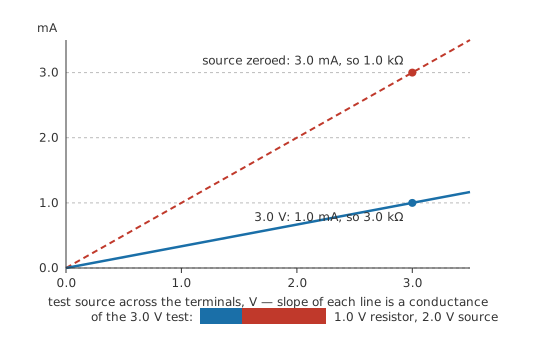
The equivalent resistance then comes from its definition rather than from the usual shortcut: deactivate the independent sources, apply a test source at the terminals, find the current it drives and take the ratio.
Worked example — Equivalent resistance with a dependent source present
The network has terminals A and B, with 1.0 kΩ from A to an internal node C, and between C and B a dependent voltage source holding C above B by 2 times the voltage across that resistor, positive terminal at C. It holds no independent source anywhere, so the open-circuit voltage is zero and only the resistance is in question.
Apply a test source of 3.0 V across A and B, A positive, and call the voltage across the resistor V_x. Walking from A to B, through the resistor and then through the source, the test voltage divides as V_t = V_x + A_v × V_x. So V_x comes to 1.0 V and C stands at 2.0 V. The test current is that V_x across the resistor, 1.0 mA, and the ratio of test voltage to test current is 3.0 kΩ.
Treat the dependent source as deactivatable and the answer comes out as the resistor on its own, 1.0 kΩ, low by a factor of 3.0. The source is opposing the test current here, which makes the terminals stiffer than the passive parts alone would suggest. Arranged to assist, it gives a resistance below anything a passive combination allows, or even a negative one, which is how a linearised transistor stage presents a negative resistance at a port.
What the equivalence requires
Linearity is the one condition the derivation actually used. Every element has to offer a proportional relationship: resistances that do not change with the current through them, ideal sources, and dependent sources of constant gain. A thermistor warming as it works, a diode, a lamp or an amplifier against its rail has no fixed equivalent, though each can be linearised about an operating point and given one that holds for small excursions around it.
The equivalence holds at the terminals and nowhere else. It reproduces terminal voltage and terminal current, and the interior it replaced takes everything else away with it: internal branch currents, internal node voltages and dissipation are all out of its reach. How far wrong the last of those goes is put into figures further down this page.
The pair of numbers belongs to one pair of terminals, too. Move them to different points on the same board and the calculation begins again, so a network has as many Thévenin equivalents as it has pairs of points.
The same line read from its other intercept gives the Norton form, a current source of V_oc ⁄ R_th in parallel with the same resistance. Source transformation converts either way, and maximum power transfer is a question asked of the equivalent.
Professional
Source resistance on the bench and in a data sheet
Characterising a source you did not design
A sealed module, a battery, a sensor board, another engineer's output stage: the equivalent of any of them is two readings and a subtraction. Measure the terminal voltage with nothing drawing current, then again with a known resistance across it. The drop, divided by the current that resistance takes, is the equivalent resistance.
Worked example — An unknown source, characterised from the outside
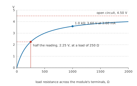
A module reads 4.50 V with nothing on its output. A 1.0 kΩ resistor across the terminals brings it down to 3.60 V, so the load is drawing 3.60 mA. That drop against that current is an equivalent resistance of 250 Ω.
The same measurement has a quicker bench form. Reduce the load until the terminal voltage reads half its open-circuit value: equal resistances share a source equally, so the load resistance at that point is the equivalent resistance. Here it happens at 250 Ω, where the terminals read 2.25 V.
Choose the load so the drop is large enough to measure and small enough to leave the source inside its normal operating region. Halving the output is comfortable on a signal source and abusive on a regulator, whose equivalent resistance is milliohms and whose behaviour changes character if you try. Take a small honest step there and accept the coarser number.
Safety
Do not measure a real source's short-circuit current to divide it into the open-circuit voltage. The division is legitimate arithmetic and the measurement is a destructive experiment: a charged battery, a mains-derived supply or a large capacitor bank can deliver hundreds of amperes into a short, welding leads and venting cells. Characterise sources with a load resistor that keeps the current inside their rating, and use a fused current path whenever you measure current at all.
The figure a data sheet already gives you
Manufacturers publish this number under several names — output impedance, source impedance, internal resistance, output resistance — and each is a Thévenin resistance quoted at the part's terminals.
A signal generator marked as having a 50 Ω output is the plainest case. Set it for 1.00 V into a matched load and its terminals carry 2.00 V with nothing connected, since the front panel is calibrated on the assumption that the load is there. Most bench generators let you tell them which assumption to use, and a wrong setting is a factor-of-two error nobody notices on a scope.
A cell's internal resistance is the same quantity, and it shows itself as a terminal voltage that sags under load and recovers afterwards. An op-amp has an open-loop output resistance that its feedback loop divides down — though never as far as zero — and that rises again as loop gain falls with frequency. A regulator publishes it as an output impedance against frequency, a curve that predicts how far the rail moves when a load switches on.
Heat belongs to the real network
Go back to the tap and its 1.0 kΩ load. The equivalent says the load takes 1.0 mW, the equivalent resistance turns 2.0 mW into heat, and the equivalent source supplies 3.0 mW. Only the first of those describes the circuit. The real supply is delivering 12.0 mW, of which the upper arm dissipates 10.67 mW and the lower arm 0.33 mW. That is 11.0 mW of heat inside a network the equivalent credits with 2.0 mW, understating it by a factor of 5.5.
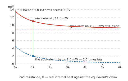
Thermal work therefore has to go back to the real network: resistor ratings, supply current budgets, heatsinking and battery runtime all belong there. The equivalent resistance is a slope taken off a graph, with no physical body behind it to get warm.
Where linearity quits
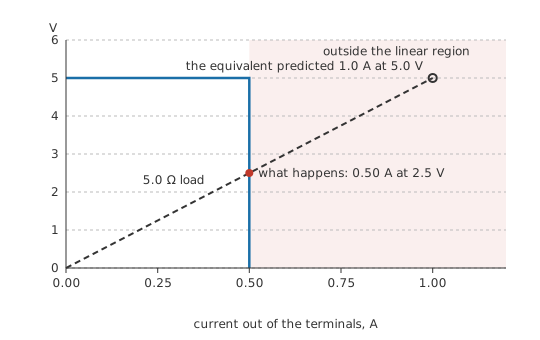
Real sources depart from their equivalents somewhere, and the departure tends to be abrupt. Current limiting is the case most bench work meets first. A supply set to 5.0 V with its limit at 0.50 A has a very small equivalent resistance while it regulates, and that equivalent predicts 1.0 A into a 5.0 Ω load. Connect the load and the supply hands over 0.50 A instead, letting its output fall to 2.5 V. That behaviour is designed in. The supply has left the region in which it was linear, and the equivalent was only ever a description of that region. A regulator dropping out as its input falls, an amplifier clipping at its rails, a discharging battery and a polyfuse on its way to opening all leave that region the same way.
Frequency is the other boundary, and everything above is DC. Where the network holds capacitance or inductance, the theorem survives with impedances in place of resistances and phasors in place of source values, and the equivalent becomes a complex quantity that moves with frequency, which is why output impedance gets published as a curve. Stray capacitance across a high-value network does this even where no capacitor was fitted.
The model stays honest in service only when the conditions travel with the numbers, since an equivalent measured at one operating point, one temperature and one load range describes that point and no other. Simulators work this way internally, linearising about an operating point to produce small-signal answers, and they will report one taken far outside the region where it means anything.
Common mistakes
- Calculating the open-circuit voltage with the load still connected. The equivalent belongs to the network alone. Take the load off first; it goes back at the very end, against the equivalent.
- "Deactivate" read as "delete". A shorted voltage source still joins its two nodes together, and that connection is often the entire reason two branches end up in parallel. Lift the part out and you have analysed a different circuit.
- Zeroing a dependent source along with the independent ones. Its value is a function of something inside the network rather than an input to it, so there is nothing there to zero. Apply a test source at the terminals and divide.
- Clipping an ohmmeter across a live circuit to read the equivalent resistance. The meter needs the sources dead and the terminals isolated, and both conditions fail on a powered board. On a network containing dependent sources no amount of deactivating would give the right answer in any case.
- A resistor rating sized from the equivalent. The equivalent resistance stands for a slope rather than a component, and it carries none of the network's heat; the figure can be out by several times in either direction. Anything thermal goes back to the real branches.
- An equivalent quoted without its terminals. A network has one equivalent per pair of points, so "the Thévenin resistance of this board" means nothing until the two points are named.
Frequently asked questions
What is the difference between a Thévenin and a Norton equivalent?
They are two descriptions of one straight line. Thévenin quotes the voltage intercept and the slope, as a voltage source in series with a resistance; Norton quotes the current intercept and the same slope, as a current source in parallel with that resistance. The current source's value is the Thévenin voltage divided by the resistance. Converting between them is source transformation, and the choice is usually whichever makes the next step of the arithmetic shorter.
Does the theorem apply to AC circuits?
Yes, with impedances in place of resistances and phasor source values in place of DC ones. The equivalent then has a magnitude and a phase, and both move with frequency, so data sheets publish output impedance as a curve instead of as a single number. Everything in this lesson is the special case at zero frequency.
My network has no independent sources at all. Is there still an equivalent?
There is: a resistance, with a zero-volt source in series that nobody bothers to draw. Finding that resistance is the interesting part once dependent sources are present, and the method is to apply a test source at the terminals and divide the test voltage by the test current. Small-signal amplifier models are analysed this way constantly.
Can I use the equivalent to find the current in a resistor inside the network?
No. The equivalent was constructed to reproduce what happens at two terminals, and it discards the rest by design. Once the terminal current is known from the equivalent, return to the original circuit, apply that current at the terminals, and solve the interior with whatever method you would have used anyway.
Why does the source resistance I measure change with the load I used to measure it?
An answer that moves means the network stops behaving linearly across the range you tested. A supply entering current limit, a battery warming or sagging, an amplifier approaching its rails and a self-heating resistance all behave that way. Narrow the measurement to a small excursion around the operating point you care about, and quote the figure with that operating point attached to it.