
Quick Answer
The superposition theorem states that in a linear circuit the voltage or current at any point equals the sum of the contributions from each independent source acting alone. Solve once per source with the rest deactivated, then add. Ideal voltage sources become short circuits, ideal current sources become open circuits, and dependent sources are never deactivated.
Intuition
One source on, the others off
A circuit with a single source can usually be worked through in a line or two of arithmetic. Put a second source into it and the standard methods — nodal and mesh analysis — still handle it, but they solve for everything at once, and the answer arrives with no record of which source produced which part of it.
Superposition works the other way about. Answer the circuit once with only the first source present, again with only the second, and add the two answers together. Every pass is a smaller problem than the one you were handed, and every result comes labelled with the source that caused it.
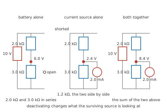
The circuit used through the rest of this lesson has one interesting node. A battery of 10 V reaches it from the left through 2.0 kΩ, and 3.0 kΩ runs from the node down to the reference rail. Feeding the same node from the rail side is a source holding a steady 2.0 mA whatever the node does.
Consider the battery on its own, with the current source disconnected and its place left as a gap in the wiring. The node stands at 6.0 V.
Reverse the arrangement — current source connected, battery taken out and replaced by a plain piece of wire — and the node stands at 2.4 V instead.
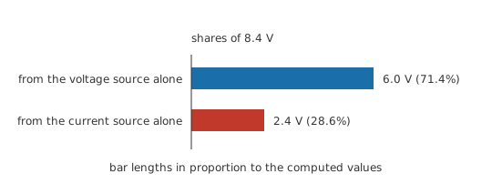
Connect both and the node sits at 8.4 V, which is the two earlier figures added. The arithmetic is exact at every step, and the agreement is general: it holds for any circuit built from resistors and ordinary sources, however many sources there are.
The wire in one pass and the gap in the other still need explaining, and so do the currents, which carry directions as well as sizes.
Practitioner
Running the circuit twice
Deactivating a source means setting to zero the quantity that source holds fixed, and what remains on the page depends on which quantity that is.
An ideal voltage source holds a fixed voltage across its terminals no matter what current passes. Set that voltage to zero and what is left is a component with no voltage across it at any current: a short circuit, drawn as a plain wire.
An ideal current source keeps a fixed current whatever voltage appears across it, so zeroing it leaves a component that carries nothing at any voltage: an open circuit, drawn as a gap.
The two rules get swapped often enough to be worth a second look, because a swap rewires the circuit. Shorting a current source joins two nodes the circuit never joined; opening a voltage source deletes a path that was carrying current.
A dependent source is left alone in every pass, without exception. Its value is a rule tying one branch to another rather than a number the circuit was handed, and that rule is part of what the circuit is. Layer 3 gives the algebraic reason.
The procedure, then:
- List the independent sources.
- Take them one at a time. Deactivate all the others and solve the reduced circuit for the quantity you want, leaving every dependent source in place.
- Record each result against a positive direction you fixed once, before the first pass.
- Add.
Each reduced circuit tends to be a series-parallel arrangement that a divider will settle without any simultaneous equations. A source feeding two arms in series is read off as a tap:
A source feeding two arms side by side needs their combination,
which fixes the node voltage,
while the branch currents come from the split, whose numerator carries the opposite branch's resistance:
Worked example — One pass per source, then an independent check
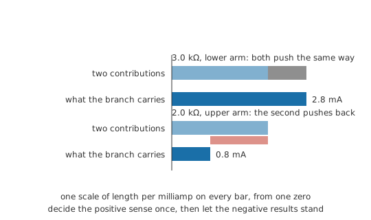
Fix the positive senses before either pass and keep them: in the upper arm, from the battery towards the node; in the lower arm, from the node towards the rail.
With the current source open, the battery sees the two arms end to end and the node is a plain tap at 6.0 V. One current runs round that loop and passes through both arms, 2.0 mA, in the positive sense in each.
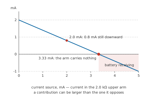
With the battery replaced by a wire, the two arms are joined at both ends and stand side by side across the current source at 1.2 kΩ, lifting the node to 2.4 V. The source's current splits between them in inverse proportion to their resistances: 0.8 mA down the lower arm, which is positive, and 1.2 mA up the upper arm towards the shorted battery, which is not.
In the lower arm the two passes push the same way and their currents add: 2.8 mA. In the upper arm they oppose, so the second contribution enters the sum negative and the total is a difference: 0.8 mA. Node voltages need none of that bookkeeping, since a voltage carries its polarity inside its own value: 8.4 V.
Now solve the untouched circuit in one step, both sources present, nothing deactivated. A current balance at the node puts it at 8.4 V, and the upper arm's current is then the battery voltage less the node voltage, over the arm's resistance: 0.8 mA. Both match the sums above.
That check confirms the arithmetic of these two passes, which is as far as any one example goes. The general guarantee comes from the theorem, and Layer 3 derives it.
Engineer
The linear system behind the theorem
Superposition belongs to linear equations rather than to circuits. Circuits inherit it because every equation used to describe one is linear.
Start with the elements. A resistance ties its voltage to its current through a constant:
Double the current and the voltage doubles; add two currents and the voltages add. Kirchhoff's two laws are linear in the same undemanding way — the currents at a node are summed with coefficients of plus and minus one, and so are the voltages round a loop. Nothing anywhere is squared, inverted or raised to a power of the unknowns.
Assemble the whole circuit and the unknown node voltages satisfy a set of simultaneous linear equations. The coefficients on the left are built from the element values and the way the parts are wired together. The right-hand side is built from the independent sources and from nothing else: a battery contributes a term, a current source contributes a term, and a resistor contributes none.
The rest of the argument is a matter of what linear systems do with a right-hand side.
Multiply that side by any number and the solution is multiplied by the same number. The property is homogeneity, and the Layer 2 circuit shows it: raise the battery from its original value to 20 V and its contribution to the node doubles, from 6.0 V to 12.0 V. The current source's contribution, untouched, stays at 2.4 V, and the node now sits at 14.4 V.
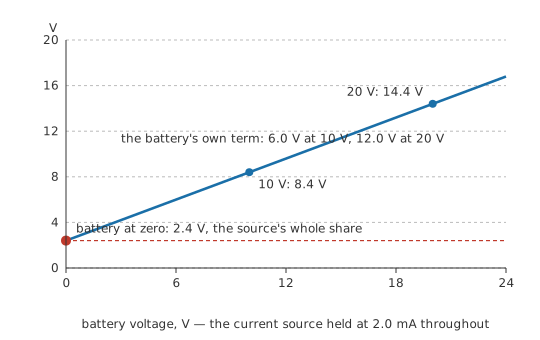
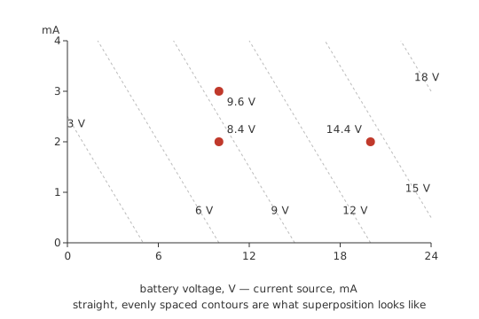
Additivity does the other half of the work. One right-hand side produces one solution and a second produces a second; put the two together and the solutions add. Bring a further source of 1.0 mA to the same node, worth 1.2 V on its own, and the node moves to 9.6 V. No pass had to be redone.
Split the right-hand side into one piece per independent source, apply additivity, and superposition falls out. Deactivating a source is what zeroing its piece looks like when you draw it: the term a voltage source contributes vanishes when its voltage is zero, which on the page is a wire, and the term a current source contributes vanishes when its current is zero, which on the page is a gap. Grouping is free as well, since the pieces can be summed in any arrangement — three sources can be handled as one pass of two plus one pass of one, if that suits the network better.
Where a dependent source sits in the algebra
A dependent source's value is proportional to a voltage or a current elsewhere in the circuit, and those are unknowns. Its term therefore belongs on the left, among the coefficients, alongside the resistances. It is a constraint linking two unknowns, and the system stays linear with it sitting there, so superposition survives dependent sources intact.
Zeroing it deletes a coefficient from the left-hand side. What that leaves behind is a different circuit, and its answers describe the different circuit rather than the one on the page.
Worked example — A dependent source through two passes
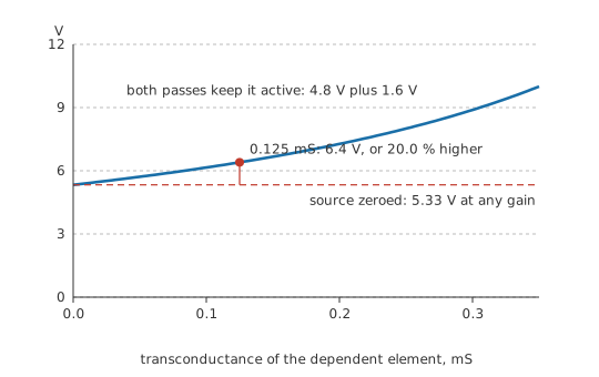
The node is fed by a battery of 12 V through 4.0 kΩ, by an independent source of 1.0 mA, and by a transconductance element whose current into the node is 0.125 mS times the node's own voltage. From the node to the rail runs 2.0 kΩ.
Both passes keep the transconductance element active. Open the independent current source and the node settles at 4.8 V. Short the battery instead and it settles at 1.6 V. The sum is 6.4 V; the untouched circuit, solved in one step, comes to 6.4 V. At that operating point the dependent element is delivering 0.8 mA of its own.
Switch it off alongside the independent pair and the same procedure, carried out just as carefully, returns 5.33 V — low by 16.7 %. The arithmetic is faultless throughout; the circuit it was performed on is the wrong one.
What the derivation assumed
The derivation asked for linearity, and it asked for it of every element without exception. Resistances must not depend on the current in them; sources must not depend on their own output; and any dependent source must be a constant multiple of its controlling quantity. A single branch that fails this removes the guarantee for the whole network.
The system also has to have one solution. A circuit with two ideal voltage sources of different values across one pair of nodes, or an ideal current source in series with an open circuit, describes an impossible situation and has no solution to superpose.
The restriction that gets overlooked most often is about what may be superposed rather than about what the circuit contains. The theorem covers quantities that are linear in the sources; voltages and currents qualify, and power does not. Layer 4 shows what that costs.
Professional
Squares do not add
The cross term
Voltage and current are linear functions of the sources, which is what lets them superpose. Power is a product of two such quantities, so it is quadratic, and a quadratic carries a term that belongs to no single source.
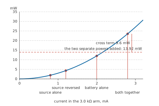
Take the lower arm of the Layer 2 circuit. The battery acting alone drives 2.0 mA through it, worth 12.0 mW. The current source acting alone drives 0.8 mA through it, worth 1.92 mW. Those two figures add to 13.92 mW.
With both sources connected the arm carries 2.8 mA and dissipates 23.52 mW. The separate powers account for 59.2 % of that.
Squaring a sum of two currents produces the square of each plus twice their product. That third piece, 9.6 mW here, is the missing amount, and because it depends on both sources at once, no calculation performed on one source at a time can produce it.
Reverse the current source and the same figures give a different answer again. Each source still drives the same magnitude through the arm, so the two separate powers are unchanged and still sum to 13.92 mW. The contributions now oppose: the node falls to 3.6 V, the arm carries 1.2 mA and dissipates 4.32 mW. One pair of separate powers therefore stands behind two true answers a factor of 3.22 apart, told apart by a sign that neither of them ever recorded.
The rule is to superpose the currents and square afterwards. The same exclusion catches efficiency, dissipation budgets and anything else assembled from a product of two responses.
A bias point with a signal on top
Superposition is the reason an amplifier can be analysed twice: once for its DC operating point with the signal set to zero, once for the signal with the supplies set to zero. The second pass is where supply rails become grounds, since a deactivated ideal voltage source is a short to the reference, which is what a decoupling capacitor is there to approximate at signal frequencies.
The circuit those two passes describe is not itself linear. A transistor is a curved device, and no amount of care makes it otherwise. What is linear is the small-signal model, a linear stand-in fitted to the curve at the bias point and valid while the excursions stay small enough for the curvature not to show. Superposition applies to the model. Small-signal is named for its condition of validity: the excursions have to stay small enough for the model to keep describing the device.
The theorem underneath the other theorems
Thévenin's theorem and Norton's are usually proved with superposition, and their working rules inherit its rules. The open-circuit voltage is a sum of contributions from the network's own independent sources. The equivalent resistance is found by applying a test source at the terminals and deactivating the internal independent sources: the same deactivation, carrying the same exemption. A network holding a dependent source must therefore be given a test source, since there is nothing in it to switch off.
One nonlinear branch is enough
A diode anywhere in a circuit ends the method. Its current is exponential in its voltage, so its branch equation is not linear, and the algebra that let contributions add is no longer available. Six perfectly linear resistors around it make no difference: the nonlinear branch enters the same system of equations they do, and the system as a whole is what has to be linear. Lamp filaments, saturating magnetic cores, varistors, amplifiers driven into their rails and any component whose value moves with the signal on it all belong to the same list.
That leaves brute force or a restriction of scope. Either solve the complete circuit numerically, as a simulator does when it iterates a nonlinear network to a solution, or linearise about an operating point, as the small-signal case above does, and apply superposition to the linearised model inside its stated range.
What the method costs
N independent sources means N analyses of the same network, so on anything large superposition costs more arithmetic than a single nodal solve. It is chosen for what it separates: supply ripple against the DC level it rides on, one interfering source among several, the share of an output error owed to each input offset. Error budgets are assembled contribution by contribution in just this way, and a measured output that nobody can account for is often traced by computing what each source alone should have produced.
Common mistakes
- Shorting the current source and opening the voltage source — the rules run the other way. A dead voltage source is a wire; a dead current source is a gap. Getting this backwards changes the topology of the network being solved.
- "A dependent source is a source, so it gets switched off with the rest." It is a constraint between two branches, and it stays active in every pass. Only independent sources are ever deactivated.
- A dissipation figure assembled from the separate passes. Power is quadratic in current, so the per-source figures omit the cross term and can land either side of the truth. Superpose the currents, then square.
- Losing a sign between passes. Fix one positive direction per branch before the first pass and score every contribution against it. Contributions recorded as bare magnitudes will add where they should have subtracted, and the working will look faultless.
- Deactivating a real source by deleting all of it. A practical source is an ideal element plus a series or shunt resistance. That resistance is an ordinary resistor and stays where it is; only the ideal element inside is set to zero.
- Reaching for superposition on a circuit containing a diode, a lamp or an amplifier at its rails. One nonlinear branch removes the guarantee for the whole network, however linear everything else is.
Frequently asked questions
Do the sources have to be taken strictly one at a time?
No. Any grouping works, so long as every independent source is accounted for once. Three sources can be handled as one pass with two of them active and a second pass with the third, which is often convenient when two supplies share a rail. The sum is the same either way.
Why can't the powers be added?
Power is a product of voltage and current, both of which are linear in the sources, so power is quadratic in them. Squaring a sum of contributions produces the individual squares plus a cross term that depends on two sources at once, and no single-source pass can generate that term. Add the currents or the voltages, then compute power from the total.
What happens to a dependent source during each pass?
Nothing at all; it stays as drawn. A dependent source is a rule relating one branch to another, so in the circuit equations it sits among the coefficients and not on the source side. Zeroing it changes the network itself instead of the excitation applied to it, and the result then belongs to a circuit that was never on the page.
Is superposition quicker than nodal or mesh analysis?
Usually not, and it is not offered as a shortcut. A network with four independent sources takes four passes, where one nodal solve would have taken one. Its value is that each answer arrives attributed to a source, which is what error budgets, interference hunts and ripple calculations need.
Does superposition work on AC circuits?
Yes, with impedances in place of resistances and phasors in place of DC values, since the element relationships stay linear. It becomes the only practical route when sources run at different frequencies: one phasor analysis cannot represent two frequencies at once, so each source is analysed at its own frequency and the time-domain results are summed. Instantaneous power still does not superpose. Average power is a special case: for sources at different frequencies the cross term averages to zero over time, so the average powers do add there, while at a shared frequency they do not.