
Quick Answer
Norton's theorem states that any linear two-terminal network behaves at those terminals like a single current source in parallel with a single resistance. The source value is the current the terminals deliver into a short circuit, and the resistance is the one Thévenin's theorem already gives, so the two equivalents describe the same network.
Intuition
A current source with a resistance across it
The theorem is about one arrangement in particular. One component pushes 6.0 mA out of itself whatever stands in its way — an ideal current source. Across it sits a resistance of 1.5 kΩ. Two wires leave the ends of that pair, and those wires are the terminals.
With nothing connected, the current has one route open to it. All of it goes through the resistance, leaving the terminals at 9.0 V.
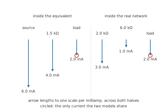
Connect a load of 3.0 kΩ and there are two routes. The current splits between them according to resistance: 2.0 mA into the load, 4.0 mA through the internal resistance, 6.0 V across both. The source is still pushing the same 6.0 mA it was pushing before. All the load has done is take a share of a total that was already fixed.
Norton's theorem raises that arrangement to a general one. Take any collection of batteries, supplies and resistances, as large as you please, and bring two of its points out to a pair of terminals. Some current source and some resistance will then behave at those terminals exactly as the network does — same terminal voltage, same terminal current, load after load — provided the parts inside behave linearly, as resistors and ordinary supplies do.
Thévenin's theorem makes the same promise with a battery and a series resistance, and both hold of one network at one time. The two forms describe one and the same behaviour, and either turns into the other in a single step.
The result carries the name of Edward Lawry Norton, an engineer at Bell Telephone Laboratories, who set it down in an internal report in the 1920s. The German engineer Hans Ferdinand Mayer described it independently at about the same time, and some texts accordingly call it the Mayer–Norton theorem.
Practitioner
Shorting the terminals to find the source
The Norton current is defined by an operation you can carry out on the network: join the two terminals with a wire, and the current in that wire is the source value — its short-circuit current, written I_N or I_sc.
That short simplifies the network before any arithmetic is done on it. Whatever bridges the terminals now holds no voltage, so any element sitting directly across them carries nothing and drops out of the calculation. What is left to solve is often a good deal smaller than the network you were handed.
The resistance is the one Thévenin's theorem already asks for, obtained the same way and with the same value. Take the load off, replace every ideal voltage source by a short circuit and every ideal current source by an open circuit, then work out the resistance seen looking back in from the terminals. On a two-arm tap, deactivating the supply joins the arms' outer ends, which leaves the arms in parallel.
Fit a load to the equivalent and the picture is one current feeding two resistances in parallel, which is the current divider. Its numerator carries the other branch's resistance, the one the current is being kept out of:
The terminal voltage then follows from either branch.
Worked example — A loaded tap, settled three ways
The network is 12 V across 2.0 kΩ above 6.0 kΩ, with the terminals at the junction of the two arms and the bottom rail. The load to be fitted is 3.0 kΩ.
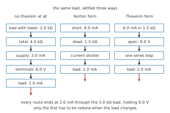
Solve it directly first, with no equivalent anywhere in the working. Once fitted, the load shares both of its nodes with the lower arm and the two combine to 2.0 kΩ; the upper arm brings the total across the supply to 4.0 kΩ, so the supply delivers 3.0 mA. That current through the combination puts 6.0 V at the terminals and 2.0 mA into the load.
The Norton route leaves the load alone until its final step. Join the terminals: the lower arm is bridged end to end, holds nothing and carries nothing, so every ampere the supply pushes through the upper arm arrives at the short. I = V ⁄ R on the upper arm alone gives 6.0 mA. Deactivate the supply and its two ends become one point, which puts the arms in parallel at 1.5 kΩ.
Hang the load on that pair. The divider sends 2.0 mA into it and leaves 4.0 mA in the equivalent resistance, with 6.0 V across both. Those are the figures the direct solve produced before the equivalent existed.
The Thévenin form is one multiplication away. A source of 6.0 mA pushing through 1.5 kΩ stands at 9.0 V with the terminals open, and that voltage behind that resistance is the series equivalent. One loop is left, and it settles at 2.0 mA, in agreement with the divider.
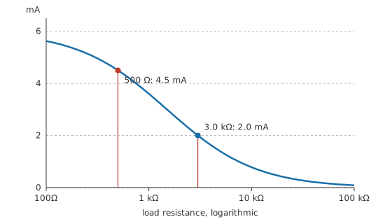
Change the load to 500 Ω and the equivalent answers without repeating any of the work: 4.5 mA into the load, 2.25 V across it. The direct route would begin again at a new parallel combination.
Conversion between the two forms runs both ways and has a name of its own, source transformation: a voltage source of V behind R becomes a current source of V ⁄ R across the same R, and back again. Applied inside a larger network it is a working move as much as a final answer, since swapping a series pair for a parallel pair often brings two resistances into a combination that will reduce.
Which form to carry depends on what comes next. A single load in series with the equivalent suits the Thévenin form, while several branches sharing one pair of terminals suit the Norton form, where each new branch simply joins the parallel group and the divider does the rest. Circuits driven by transistors, photodiodes and current-output converters arrive as Norton sources already, and the last section of this lesson takes them up.
Engineer
One line, read from its other end
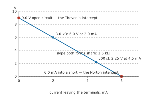
A linear network can present only a straight line at its terminals. Plot terminal voltage against the current leaving the terminals; every load you might connect puts a point somewhere on that one line. The load decides where on that line the circuit sits, while the line itself is the network's property.
A line is fixed by an intercept and a slope, and it has an intercept on each axis, so it can be named in either of two ways. Take the voltage intercept with the slope and you have written V = V_oc − I R_th, a voltage source behind a resistance. The current intercept with the same slope gives I = I_N − V ⁄ R_N, a current source with a resistance across it. Both namings are on the same footing, and since the slope belongs to the line, the resistance in the two forms is one number appearing twice.
Reading the conversion off the line
Put V at zero in the first form and the current comes to V_oc ⁄ R_th, which is what shorting the terminals delivers, so I_N = V_oc ⁄ R_th. Setting I to zero in the second leaves the voltage at I_N R_N, the open-circuit value. Any two of the three fix the third. The worked network's 9.0 V and 6.0 mA sit at the ends of one line of slope 1.5 kΩ, with the loaded point at 6.0 V and 2.0 mA between them.
The duality between the forms is thorough, and reading it off takes no more than the substitutions. Series becomes parallel, a voltage source becomes a current source, an open circuit becomes a short circuit, and the operation that finds one intercept becomes the operation that finds the other. Every statement true of one form has its partner in the other, so Thévenin's derivation carries over here intact, conditions and algebra together.
A third reading of the same geometry supplies the resistance directly. It is the ratio of the two intercepts, V_oc ⁄ I_sc, so computing both and dividing produces it while every source in the network stays live. That route matters where deactivation is not permitted. A dependent source takes its value from a voltage or current inside the network, so setting it to zero deletes one of the equations that define the circuit; superposition makes the same exception, since its sum runs over the independent sources alone. The ratio route does need one independent source somewhere. Where a network has none, both intercepts are zero, the ratio says nothing, and the resistance comes from a test source applied at the terminals.
Choosing the route with less work in it
Both intercepts describe the same line, and one is usually a good deal cheaper to compute than the other. Which one depends on the network, and the gap can be wide in either direction.
Worked example — A ladder, where the open-circuit route is the short one
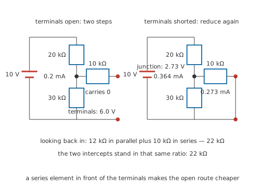
The supply is 10 V across 20 kΩ above 30 kΩ, and 10 kΩ runs from that junction out to the terminals.
With the terminals open, no current passes through the third resistor, so it drops nothing and the terminals report whatever the first two arms leave at their junction. A loop current of 0.2 mA across the lower arm puts 6.0 V at the terminals, and the third resistor never entered the working.
Short the terminals and it stops being a bystander. It now stands in parallel with the lower arm at 7.5 kΩ, which the upper arm sees as a total of 27.5 kΩ. Supply current becomes 0.364 mA, the junction falls to 2.73 V, and the short carries 0.273 mA. Every interior figure moved, and the reduction had to be done again from the start.
The resistance comes out the same by either road. With the supply shorted, the first two arms are in parallel at 12 kΩ and the third is in series with that pair: 22 kΩ. The two intercepts stand in the same ratio, 22 kΩ.
Worked example — A node fed from three branches, where the short is the shortcut
Here the terminals are one node and the reference rail. Arriving at that node are 12 V through 4.0 kΩ, an ideal source pushing 2.0 mA, and 6.0 V through 2.0 kΩ; a further 4.0 kΩ runs from the node down to the rail.
Join the terminals and the node is pinned to the reference. Each supply branch now has its whole source voltage across its own resistance and nothing else in its way, so each contributes on its own: 3.0 mA from the first, 3.0 mA from the third, the current source handing over its 2.0 mA unchanged, and the shunt carrying nothing at all. They add to 8.0 mA. That addition would still be the only step required however many branches met at that node.
The resistance comes from the same drawing with the sources dead: the two supply resistances and the shunt in parallel, 2.0 kΩ for the first pair and 1.0 kΩ once the third joins them. Wanting the open-circuit voltage first would have meant writing the node equation that shorting made unnecessary, for an answer of 8.0 V.
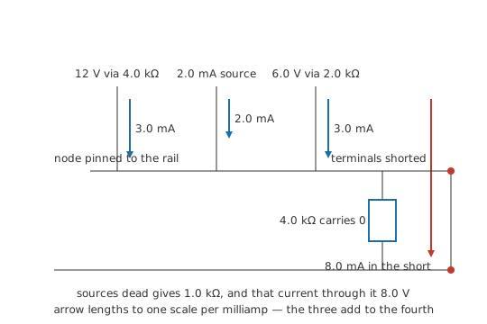
A working habit falls out of the pair. A network whose sources all reach the terminals through resistances meeting at the terminal node gives up its short-circuit current by inspection, because the short pins that node and each branch then contributes on its own. A network with a series element in front of its terminals hands over its open-circuit voltage far more readily, because that element stays idle until something shorts the terminals. Look at which shape you have before starting, and take the remaining intercept from the ratio.
How far the equivalence reaches
Linearity is the condition, the same one Thévenin's theorem needs and for the same reason: a linear network is what produces a straight terminal characteristic, and a straight line is what two numbers are enough to describe. Resistances that change with the current in them, diodes, filament lamps and amplifiers against their rails have no fixed equivalent, though each can be linearised about an operating point and given one that holds for small excursions near it.
Equivalence holds at the terminals and nowhere else. The pair reproduces terminal voltage and terminal current, which is all it was ever asked to do, and the interior stayed behind in the network it replaced. Branch currents and node voltages inside it, along with any dissipation figure, have to be looked for there rather than in the two components standing for it. The current the model shows in the equivalent resistance is a bookkeeping remainder that no component in the real network carries. The pair belongs to one pair of terminals, too, so a network has as many Norton equivalents as it has pairs of points.
The duality breaks at either ideal extreme. An ideal voltage source alone has zero equivalent resistance and an unbounded short-circuit current, so no Norton form exists for it; an ideal current source alone has infinite equivalent resistance and no open-circuit voltage, so it has no Thévenin form. Real sources sit far enough from both for this to be a statement about idealisations, and it surfaces in practice when a simulator refuses to converge on a circuit holding an ideal source with nothing in series or parallel with it.
Professional
Devices that are current sources to begin with
A photodiode delivers a current
A photodiode passes a current proportional to the light falling on it, with a large shunt resistance across it — a Norton source whose two elements are both quoted on the data sheet, one as responsivity and one as shunt or dark resistance. The proportionality holds while the terminal voltage stays near zero, which is the condition the measuring circuit exists to maintain.
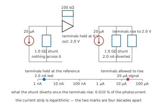
A photocurrent of 20 µA into an op-amp stage whose feedback resistance is 100 kΩ, with the loop holding the diode's terminals at the reference, gives an output of 2.0 V. The whole photocurrent crosses to the feedback resistor because the branch it would otherwise share with — the shunt resistance — has nothing across it.
Load the diode with a resistor instead and its terminals rise. At 2.0 V across a shunt resistance of 1.0 GΩ, the shunt takes 2.0 nA, or 0.010 % of the photocurrent. That is small at room temperature and at this signal level, and it grows with both, which is the argument for holding the terminals at zero volts and letting the amplifier convert.
The two intercepts on a solar cell's data sheet
A photovoltaic cell's data sheet gives a short-circuit current and an open-circuit voltage: the two intercepts, named as such. Take 500 mA and 0.60 V. Their ratio comes to 1.2 Ω, a figure the cell's own characteristic matches nowhere along its length.
The characteristic bends. It stays close to the short-circuit current across most of the voltage range and then collapses near the open-circuit end — a knee — so the two quoted numbers are the two ends of a curve rather than the intercepts of a line. Equivalents exist for linear networks only, and the useful operating point sits inside the knee, away from both quoted figures. The same caution applies to maximum power transfer, whose matched-load result was derived from a linear equivalent and does not locate a solar cell's maximum-power point.
Collector current with a resistance across it
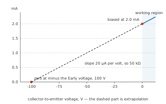
A bipolar transistor in its active region passes a collector current set by its base and nearly independent of its collector voltage, which is what a current source is. The "nearly" is the Early effect, and it gives the collector a finite output resistance. At 2.0 mA with an Early voltage of 100 V, that resistance is 50 kΩ.
A current in parallel with a resistance is a Norton equivalent, and it is the form the small-signal model of a stage uses at the collector. Whatever load is hung there joins the parallel group, and the divider gives the answer without the model being rearranged.
Why a current output prefers a small load
A current-output converter has the same shape. Full scale of 2.0 mA behind an output resistance of 10 kΩ, driven into a 1.0 kΩ resistor, delivers 1.82 mA to that resistor, which is 9.09 % short of full scale, and the shortfall moves with the load. Hold the output at a virtual earth and the load resistance is near enough zero that the divider hands over the whole current and the output resistance stops mattering.
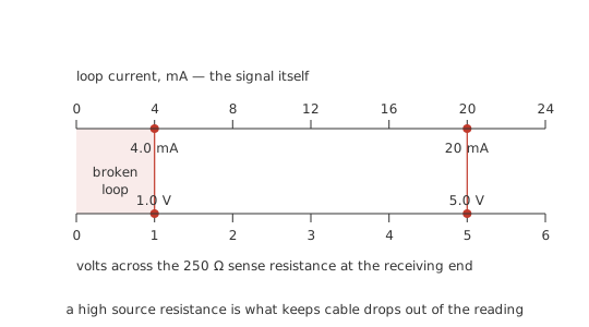
Industrial transmitters exploit the same property over long distances. In a 4–20 mA loop the measurement is the current, sent by a transmitter whose output resistance is very high, so cable resistance and drops along the run do not enter the reading. At the receiving end a sense resistance of 250 Ω turns 4.0 mA into 1.0 V and 20 mA into 5.0 V, and the live zero at the bottom of the range separates a genuine reading of nothing from a broken wire.
Getting the two numbers off a real source
Norton's two numbers are the harder pair to get out of a real source. An open-circuit voltage costs nothing to obtain — a meter across the terminals draws microamperes and disturbs almost nothing. A short-circuit current asks you to short the source, and on a bench supply, a battery or a charged capacitor bank that experiment gives a wrong answer at best and a welded lead at worst.
Even where the current is small enough to be harmless, the reading is often something other than the intercept you wanted. A supply in current limit, an amplifier at its output-current ceiling and a cell sagging under a heavy load have all left the region in which they were linear, and the number they hand back belongs to no straight line.
Bench practice therefore characterises sources in Thévenin form — an open-circuit reading and one reading with a known load — and converts to Norton on paper when the next step wants it. The Norton form is the cleaner one to analyse and the more awkward one to measure. Those are two separate facts about a single equivalent, and an engineer who remembers both keeps the model tied to the source it stands for.
Safety
Every short-circuit current quoted in this lesson is a division performed on component values, and no source was shorted to produce one. Do not short a real source to find its Norton current. A battery, a mains-derived supply or a charged capacitor bank can deliver hundreds of amperes into a short — welded leads, vented cells, burns and fire — and even sources that survive it will have left their linear region, so the reading is worthless as well as dangerous. Measure the open-circuit voltage and one loaded point instead, keep the current inside the manufacturer's rating, and fuse any path you measure current through.
Common mistakes
- Reading the Norton current as the current the load will receive. It is the current into a short across the terminals, the largest the network can deliver. Every real load takes less, since the equivalent resistance keeps a share of it.
- "Two equivalents, so two sets of measurements." One set gives both. The resistance is common to them, and either intercept produces the other through it in a single step.
- Zeroing a dependent source alongside the independent ones. Its value is a function of something inside the network and there is nothing there to set to zero. Divide the two intercepts, or apply a test source at the terminals.
- A current-divider numerator taken from the branch being solved for. The load current is the total times the opposite branch's resistance over the sum of the two. Written the wrong way round it hands the larger current to the larger resistance — the check to run whenever a divider answer looks upside down.
- Shorting a real source's terminals to obtain the Norton current. The operation is a paper one. On the bench, take an open-circuit reading and one loaded reading and convert.
- Sizing a component from the current the model shows in the equivalent resistance. No part of the real network carries it. Anything thermal goes back to the actual branches.
Frequently asked questions
How do I convert a Norton equivalent into a Thévenin equivalent?
Keep the resistance and multiply. The Thévenin voltage is the Norton current times the shared resistance, and the two components go from parallel to series. Going the other way, the Norton current is the Thévenin voltage divided by that same resistance. The move is called source transformation, and it is an exact identity.
Which equivalent should I look for on a given network?
Whichever intercept the network gives up more cheaply. Sources reaching the terminals through resistances that meet at the terminal node favour Norton, since shorting the node lets each branch contribute on its own and the contributions add. Terminals sitting behind a series element favour Thévenin, since that element carries nothing until the terminals are shorted. Take the intercept you did not compute from the ratio of the other two.
Does every network have a Norton equivalent?
Every linear one does, with a single exception at the ideal end. An ideal voltage source with nothing in series has zero equivalent resistance and an unbounded short-circuit current, so no Norton form exists for it; the mirror case is an ideal current source, which has no Thévenin form. Nonlinear networks — anything built around diodes, lamps or a saturating amplifier — have no fixed equivalent of either kind, only a linearised one that holds near a stated operating point.
Can I work out the heat in the original circuit from its Norton equivalent?
No. The equivalent reproduces what happens between two terminals and keeps no record of the interior, so the current it shows in the equivalent resistance is bookkeeping and not a current any component carries. Return to the real network with the terminal current known, and size ratings there.
Does the theorem work on AC circuits?
It does, with impedances in place of resistances and phasor values in place of DC ones. The Norton current then has a magnitude and a phase, the parallel element is a complex impedance, and both move with frequency, so an output impedance is published as a curve rather than as a single number.