
Quick Answer
Source transformation exchanges a voltage source in series with a resistance for a current source in parallel with the same resistance, and back again. The current value is the source voltage divided by that resistance. Applied repeatedly inside a network, it collapses arrangements that series-parallel reduction alone cannot touch. The equivalence holds at the terminals only.
Intuition
A load cannot tell the two apart
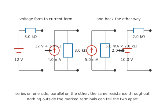
Put a 12 V battery in series with a 3.0 kΩ resistor and bring the two free ends out as a pair of terminals. Beside it, set up a source that pushes a steady 4.0 mA into whatever it meets, with a second 3.0 kΩ resistor straight across it, and bring those ends out as terminals as well. The two arrangements have no component in common and look nothing alike on a page, and different things go on between their terminals.
Connect nothing to either, and both pairs of terminals give the same reading. With no current anywhere in the series pair, its resistor drops nothing and the terminals show the battery's own 12 V. In the parallel pair every ampere the source produces has nowhere to go but the resistor, which stands the terminals at 12.0 V.
Now hang 1.0 kΩ on each. The series arrangement offers one loop of 4.0 kΩ carrying 3.0 mA, leaving 3.0 V across the load. In the parallel arrangement the load joins the resistor already sitting there, the two coming to 750 Ω, and the source current crossing that combination leaves 3.0 V at the terminals with 3.0 mA in the load. The readings match again, and they go on matching for any load you care to substitute.
Source transformation is the licence to swap one arrangement for the other. Thévenin's theorem and Norton's between them establish that both descriptions exist for any linear network. This lesson is about performing the swap partway through a calculation, while the network is still being reduced.
Practitioner
One multiplication each way
Going from the voltage form to the current form, the current value is what the source voltage drives through its own series resistance, V ⁄ R, which is also the current the terminals would deliver into a short circuit. The reverse direction multiplies instead: the source current develops I × R across its own parallel resistance, and that product is the voltage the open terminals would show. Neither direction is more than a line of arithmetic.
The resistance itself carries over untouched. Its position changes, from in line with the source to across it, while its value stays exactly where it was; there is nothing about it to recompute.
Polarity travels with the value, and this is where the swap is most often fumbled. The current source's arrow points the way the voltage source's positive terminal pushed current out into the external circuit. Going back the other way, the positive terminal lands on the side the arrow was aiming at. A quick check settles it: work out the terminal voltage of both versions under one small load and confirm that the signs agree as well as the magnitudes.
Whichever form is on the page, the terminals obey one straight characteristic: an open-circuit voltage, falling as current is drawn, at a rate the resistance fixes.
Loading the voltage form is a loop problem: add the resistances and divide into the source voltage. The current form makes it a node problem instead, where the two resistances go side by side before anything is multiplied.
Worked example — Converted, loaded, and converted back
The source on the page is 5.0 mA in parallel with 2.0 kΩ, and the load waiting to be fitted is 3.0 kΩ.
Leave the terminals open and the whole source current crosses its own parallel resistance, so V = I × R gives 10.0 V. That figure in series with the same 2.0 kΩ is the voltage form, positive terminal on the side the arrow pointed.
Fit the load to it. Two resistances in a row make 5.0 kΩ, the loop carries 2.0 mA, and the terminal voltage is the source voltage less what the internal resistance takes from it: 6.0 V.
Now put the same load on the original current form. Load and internal resistance share both of their nodes, combining to 1.2 kΩ, and the full 5.0 mA crosses that combination for 6.0 V at the terminals and 2.0 mA in the load. The two routes share no arithmetic and arrive at the same figures.
Convert back and the original returns exactly: 10.0 V across 2.0 kΩ is 5.0 mA, the value the swap started from. Both steps are exact identities, which is why a round trip accumulates no error.
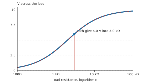
Which way to convert is settled by the shape of the next step. A single load sitting in line with the source is a loop, and the voltage form hands it over directly. Where several branches meet at one pair of nodes, the current form lets each new branch join the parallel group where it stands.
Engineer
Transform, combine, transform back
Two supplies feeding one load through separate resistances hold no series pair and no parallel pair, so series-parallel reduction has nothing to start on. Nodal or mesh analysis will settle such a network, at the price of setting up and solving an equation.
The transformation offers another route, and it can be applied again to its own output. Convert both voltage sources and their two internal resistances, which shared no node a moment ago, now hang between the same two nodes. Resistances in parallel combine and parallel ideal current sources add, so two branches have become one. A single transformation back puts the result in the form the load wants.
Worked example — Two supplies, reduced by transforming twice
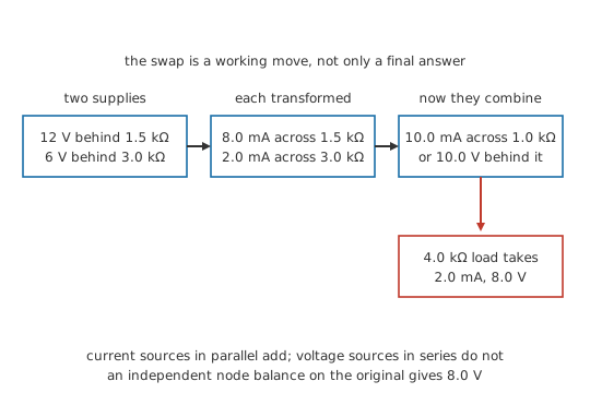
12 V reaches the node through 1.5 kΩ, 6 V reaches the same node through 3.0 kΩ, and 4.0 kΩ runs from that node down to the rail.
Transform both supplies. The first becomes 8.0 mA with 1.5 kΩ across it, the second 2.0 mA with 3.0 kΩ across it, and all four elements now stand between the node and the rail.
Combine what the transformation has just put side by side. The two source currents add to 10.0 mA, and the two resistances in parallel come to 1.0 kΩ. That leaves one source and one resistance, with the load still untouched.
Transform back. 10.0 mA through 1.0 kΩ stands at 10.0 V, now in series with that same 1.0 kΩ, so fitting the load closes a single loop of 5.0 kΩ. The loop carries 2.0 mA and the load holds 8.0 V.
The sequence needed arithmetic only, never a simultaneous equation, and the load was fitted once, at the end. As a check, balance the currents arriving at the node against the current leaving through the load, with the original circuit untouched and nothing transformed anywhere: 8.0 V.
The reduction generalises. Three supplies reaching one node through three resistances collapse the same way, all three currents adding and all three resistances combining. A chain of alternating series and shunt elements can be walked from the far end towards the terminals, transforming at each step, and a bridge that has resisted every attempt at reduction sometimes yields once one arm has been rewritten in the other form.
The node that disappears
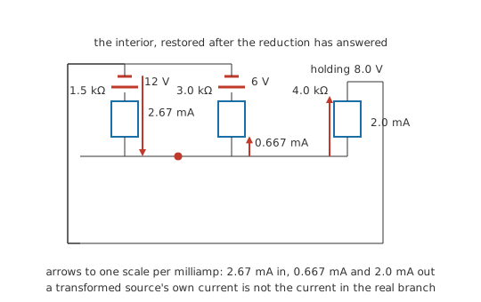
Each transformation costs a node. The junction between the first supply and its resistance existed before the swap and does not exist after it, so any current or voltage belonging to that junction has left the model along with it.
Those figures come back afterwards, one subtraction at a time, once the terminal voltage is known. In the worked network the first resistance carries 2.67 mA, the difference between its supply and the node divided by its own value. The second carries 0.667 mA in the opposite sense, flowing into the 6 V supply rather than out of it, since the node ends up above that supply's voltage. Both follow ordinarily from the answer, though the reduced circuit that produced it has no room for them.
The same warning has a stricter form. A transformation may only absorb a resistance that is genuinely in series with its source, meaning nothing else is connected to the junction between them. Attach a third branch to that junction and the pair is no longer a source with a series resistance; it is a three-way node, and swapping it for a current source would delete a connection the circuit actually has.
The swap needs a resistance in the right place
An ideal voltage source with no series resistance has no current-source equivalent. The conversion asks for the source voltage divided by zero ohms, and the infinity it returns is real: the arrangement holds its voltage into a short while supplying unbounded current, which no finite current source does. The mirror case is an ideal current source with nothing in parallel with it: its open-circuit voltage is unbounded, so no finite voltage source stands in for it. Real sources always carry some series or shunt resistance, which is why the difficulty shows up mainly in idealised paper circuits and in a simulator refusing to converge.
Ideal sources permit a deletion of their own. A resistance in parallel with an ideal voltage source has no effect on anything outside it, since the source holds the voltage regardless, so it can be struck out before the swap. A resistance in series with an ideal current source is equally inert, since the current is fixed regardless of what stands in its way. Both deletions change the interior of the network and leave every external quantity where it was, which is the same bargain the transformation itself offers.
Linearity is the underlying condition, inherited from the two theorems this method is built on. Where a branch fails it — a resistance moving with its own current, a diode, a lamp filament, an amplifier at its rails — neither equivalent exists in fixed form.
Professional
The inside of the model is not equivalent
Identical terminals, different heat
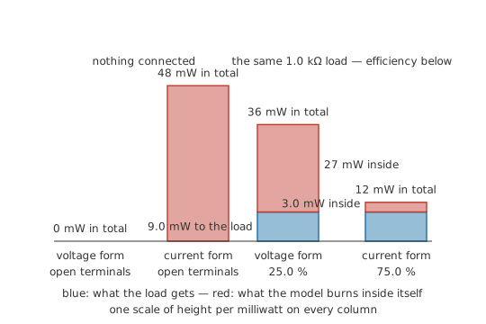
Return to the pair of arrangements the lesson opened with and leave both sets of terminals open. The series form carries no current at all, so its resistance dissipates 0.0 W. The parallel form has its entire 4.0 mA circulating through 3.0 kΩ, dissipating 48 mW while its terminals sit at the same voltage and deliver nothing.
Loading them narrows the gap without closing it. With 1.0 kΩ connected, both deliver 9.0 mW to the load. The series form's internal resistance carries the load current and dissipates 27 mW; the parallel form's carries only the share the load left behind, 1.0 mA, worth 3.0 mW. A factor of 9.0 separates two models that no external measurement distinguishes. The totals drawn differ to match: 36 mW against 12 mW, so the same delivered power arrives at 25.0 % efficiency in one model and 75.0 % in the other.
Neither figure belongs to a real component unless the model happens also to be the real circuit. Terminal voltage, terminal current and anything computed from the two are exact. Dissipation, efficiency, temperature rise and component ratings are questions about the interior, and the interior was never the thing being reproduced. Take the terminal result back to the actual branches and size parts there.
A rail and a resistor, used as a current source
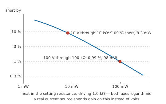
The transformation also gets built rather than drawn, and usually built badly. A 10 V rail behind 10 kΩ is treated as a 1.0 mA current source, which is the voltage-to-current conversion carried out with real components. It works to the extent that the load is small beside the setting resistance. Put 1.0 kΩ in that circuit and the current is 0.909 mA, low by 9.09 %.
Improving it costs voltage and heat in the same proportion. Raise the rail to 100 V behind 100 kΩ for the same nominal current, and the same load now sees 0.990 mA, low by 0.99 %. The error has come down by roughly a factor of ten; the setting resistor's dissipation has gone from 8.3 mW to 98 mW, and the circuit has acquired a rail that needs respect. This is the arrangement behind an LED's series resistor, and the accuracy above is why that part is called a current limiter rather than a current source.
Safety
The higher-rail comparison above was worked through with component values and a calculator, and no supply was ever set to that voltage. Direct-current rails above roughly 60 V are hazardous to handle, and a bench supply at that setting deserves the same care as mains: probe with rated leads, keep one hand off the bench, and discharge any capacitance before touching the circuit.
Why the real thing is an active circuit
A genuine current source raises its output resistance without raising its supply rail, and doing that takes gain. A transistor in its active region already passes a collector current largely independent of collector voltage. A current mirror copies a reference current into a load, and an op-amp wrapped around a sense resistor forces the load current to track a control voltage, correcting whatever the load does. All three behave like a Norton source with megohms of output resistance running from a modest supply, and all three are circuits rather than single parts.
The analysis proceeds unchanged. The small-signal model of such a stage is a current source with a resistance across it, which transforms exactly like any other. The dependent sources used to model amplifiers behave the same way: a dependent voltage source with a series resistance becomes a dependent current source with the same parallel resistance, provided the controlling quantity does not live on the node the swap is about to consume.
Common mistakes
- Recalculating the resistance during the swap. It moves from in-line to across, or the reverse, and keeps its value throughout. A new number there means the arithmetic has drifted onto some other network.
- "The source is rated for the full current, so the load receives it." The parallel resistance takes a share of that current at every load, and the load takes what is left over. Only a short across the terminals collects the whole of it.
- A dissipation figure read off the transformed model. The two forms produce different internal heat from identical terminal behaviour, so ratings and temperature rises have to be worked out in the real branches. This is the error that survives longest, because the terminal answers it sits beside are correct.
- Transforming across a junction that has a third branch attached. The resistance has to be in series with its source and connected to nothing else, or the swap deletes a real connection.
- The arrow pointing the wrong way after the conversion. Everything downstream then comes out with a plausible magnitude and a reversed sign. Fix the direction against the original polarity before the next step, since later steps will not reveal it.
- Reaching for the transformation on an ideal source with no resistance beside it. There is nothing to absorb, and the conversion produces zero or infinity. Real sources come with an internal resistance, so this is a difficulty of idealised drawings.
Frequently asked questions
Is source transformation the same thing as Thévenin and Norton equivalence?
It rests on both, and it is used differently. Thévenin's and Norton's theorems are statements that a two-terminal network has a two-component equivalent, usually applied once, at the end, to a network you are finished with. Source transformation applies the same equivalence to a single source and its resistance in the middle of a network, repeatedly, as a way of getting the rest of the circuit to reduce.
Which direction should I convert in?
Convert towards whatever the next simplification needs. Elements that will end up sharing both nodes want the current form, where parallel resistances combine and parallel source currents add. A single load in line with the source wants the voltage form, where one loop finishes the job. On a long chain it is normal to alternate, converting in one direction, combining, then converting back.
Does the resistance have to be a physical resistor?
No. It can be a combination already reduced from several parts, a source's internal resistance, or a Thévenin resistance obtained from a larger network — any resistance correctly in series with the voltage source or in parallel with the current source. Whatever it stands for, the transformation moves it without changing its value.
Can a dependent source be transformed?
Yes, by the same rule and with the controlling expression carried across unchanged. A dependent voltage source with a series resistance becomes a dependent current source with that resistance in parallel, its value divided by the resistance. The one restriction is that the controlling voltage or current must not belong to the node or branch the swap removes, since that quantity would no longer exist to be referred to.
Does it work on AC circuits?
It does, with impedances in place of resistances and phasors in place of DC values. A voltage phasor in series with an impedance becomes a current phasor of the same value divided by that impedance, in parallel with it, and both quantities are complex. The equivalence is still confined to the terminals, and the reactive elements inside the two forms store and dissipate differently.