
Quick Answer
A dependent source, or controlled source, is a voltage or current source whose value is set by a voltage or current somewhere else in the same circuit. The four types are distinguished by which quantity controls and which is delivered: VCVS, VCCS, CCVS and CCCS. They are how active devices are modelled.
Intuition
The value that is written as a rule
Up to here, a source drawn on a schematic has arrived with a number attached: nine volts, twenty milliamps. You read the number off the drawing and used it, and nothing else in the circuit could alter it.
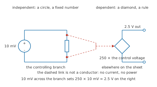
A dependent source — the older name controlled source means the same thing — carries an instruction in place of a number. Beside it you find something like two hundred and fifty times the voltage across R3. Until you know what R3 is doing, this source has no value. Work out the voltage at R3 and the source's value follows immediately; change the circuit so that voltage halves, and the source's output halves with it.
A source like that therefore straddles the drawing. Its output appears at one pair of terminals, while the branch or node whose voltage or current does the controlling can sit some distance away on the sheet. The link between them is not a wire and carries no power; what it records is how one quantity is worked out from another.
Independent sources — batteries, bench supplies, signal generators — impose their value on the circuit around them and hold it. Dependent sources are the reverse arrangement, and they exist because the components that made electronics interesting behave exactly this way. A transistor's output current follows whatever you do at its input, and an op-amp output voltage follows the difference between its two inputs. Drawing the model of an amplifying device means drawing a dependent source.
On a schematic the shape usually tells you which kind you are looking at: a diamond outline for a dependent source, a circle for an independent one.
Practitioner
Four types, four different gain units
Each of the four names states the controlling quantity first and the delivered quantity second, so a voltage-controlled current source is controlled by a voltage and delivers a current.
- VCVS — voltage-controlled voltage source. Its gain is a voltage gain, volts out per volt in, so it is a pure number with no unit.
- VCCS — voltage-controlled current source. Its gain is a transconductance, amperes out per volt in, measured in siemens and nearly always written g_m.
- CCVS — current-controlled voltage source. Its gain is a transresistance, volts out per ampere in, measured in ohms.
- CCCS — current-controlled current source. Its gain is a current gain, amperes out per ampere in, so again a pure number.
Each gain's unit is fixed by the conversion that source performs. A transconductance turns volts into amperes, so it comes out in amperes per volt, which is the siemens; a transresistance works the other way round and lands in volts per ampere, which is the ohm. Quote a gain with its unit and any dimensional slip further down the working announces itself.
The current-controlled pair follow the same shape with the roles swapped: a CCVS multiplies its controlling current by a transresistance to produce a voltage, and a CCCS multiplies its controlling current by a dimensionless gain to produce a current.
Worked example — One control signal each, four outputs
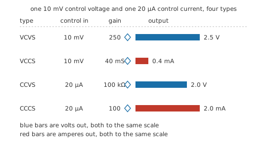
All four types are driven from the same pair of control signals: a voltage of 10 mV where the type accepts a voltage, and a current of 20 µA where it accepts a current.
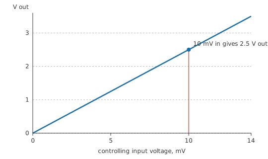
The VCVS has a voltage gain of 250, so its output is 2.5 V. Give the VCCS a transconductance of 40 mS and what appears at its output is a current instead: 0.4 mA.
On the current-controlled side, a transresistance of 100 kΩ turns the control current into 2.0 V at the CCVS output, while a current gain of 100 turns the same control current into 2.0 mA at the CCCS output.
The load is missing from all four figures, and deliberately so. A dependent source is still an ideal source, holding its output whatever is connected across it, with compliance that never runs out. Its value now comes from elsewhere in the circuit, and that is the only property the dependence changes.
You do not buy a dependent source, and there is no part number for one. Where it turns up is inside the model of a real device: an op-amp is treated as a VCVS with an enormous voltage gain, a bipolar transistor as a VCCS to first order, and the same transistor in h-parameter form as a CCCS whose gain is the base-to-collector current gain. The photodiode front end that converts a tiny current into a usable voltage is, in behaviour, a CCVS. Simulator netlists are its other home, and there all four types exist as elements you can write down directly — the subject of circuit simulation.
Spotting which quantity is doing the controlling is the practical skill when you read one of these off a schematic. Follow the two control terminals to wherever they land, identify the voltage or current there, and one multiplication gives you the source's value.
Engineer
Linear, and never switched off
The relationship a dependent source enforces is a constant multiplied by one circuit variable. That is a linear relationship, and it is the reason the rest of this department survives contact with active devices: a network of resistors, independent sources and linear dependent sources is a linear network, so superposition, Thévenin's theorem, Norton's theorem, nodal analysis and mesh analysis all remain valid, unmodified. Linearity is the only thing any of them ever asked of the sources in a network. If a source's output were instead proportional to the square of a circuit variable, or to the product of two of them, the network would not be linear and none of those tools would apply.
One step in those methods does have to be handled differently, and it is where most of the marks are lost. Superposition and the shortcut route to Thévenin resistance both proceed by deactivating sources: replacing each voltage source with a short and each current source with an open. That step applies to independent sources only. A dependent source is never deactivated. It is a constraint the network places on itself rather than an excitation applied to it from outside, so it stays in force through every sub-analysis, obeying its rule and responding to whatever the controlling variable happens to be in that sub-circuit.
The immediate consequence is that Thévenin resistance can no longer be obtained by killing the sources and collapsing the resistor network. Instead you apply a test source at the terminals — a test voltage and measure the current it supplies, or a test current and measure the voltage that appears — and take the ratio. The alternative is to compute the open-circuit voltage and the short-circuit current from the intact circuit, with all sources present, and divide one by the other.
Worked example — Thevenin resistance with the controlled source alive
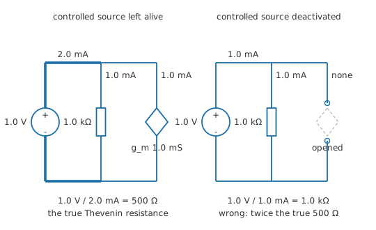
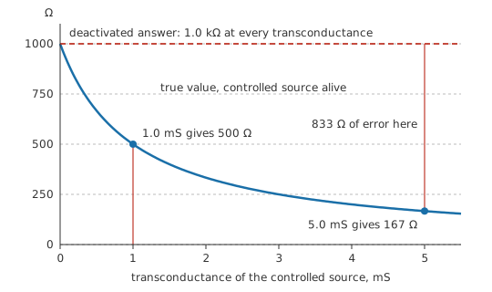
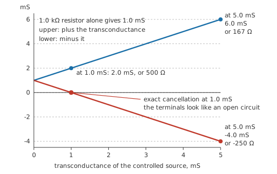
A small network presents a resistor of 1.0 kΩ across its terminals, alongside a voltage-controlled current source of transconductance 1.0 mS that draws current into the network and is controlled by the terminal voltage itself. No independent source is present anywhere in it.
Apply a test voltage of 1.0 V across the terminals. The resistor takes 1.0 mA. The controlled source sees that same terminal voltage as its controlling variable and takes 1.0 mA as well, so the test source must supply 2.0 mA altogether. Test voltage divided by test current is the Thevenin resistance: 500 Ω.
Deactivate the dependent source instead — open-circuit it, as you would an independent current source — and only the resistor is left, giving 1.0 kΩ, double the correct value. That error does not shrink as the numbers change. Raise the transconductance and the true resistance falls further, while the deactivated answer stays exactly where it was.
Nodal and mesh analysis need one addition rather than a change of method. Write the node or loop equations as usual, treating the dependent source's value as a symbol; then add one constraint equation for each dependent source, expressing its controlling variable in terms of the unknowns you are already solving for. A source controlled by the voltage across a resistor becomes a difference of two node voltages; a source controlled by a branch current becomes that current written in terms of node voltages. Each dependent source adds one unknown and one equation, so the system stays square and solvable.
The control link itself still carries no power. The source is a different matter: a dependent source can deliver net power into the rest of the network. In the real device that energy arrives from a bias supply which the model, being a model of small changes only, does not show. A network containing a dependent source is therefore not passive, and its Thévenin resistance is not guaranteed to be positive — arrange the control so the source pushes current out as the terminal voltage rises and the ratio comes out negative. Negative resistance of that kind is a genuine physical effect: it is the mechanism behind oscillators, and the reason an amplifier with feedback can be made to sing.
Professional
Where the gain number comes from
Dependent sources reach practising engineers almost entirely through small-signal models. The hybrid-pi model of a bipolar transistor is a VCCS: an output current equal to a transconductance times the base-emitter voltage, with resistors and capacitors around it. The h-parameter model of the same transistor is a CCCS driven by the base current. An op-amp macromodel opens with a VCVS of enormous gain, and a MOSFET at low frequency is again a VCCS. Between them, those four abstract types cover essentially every active device in service.
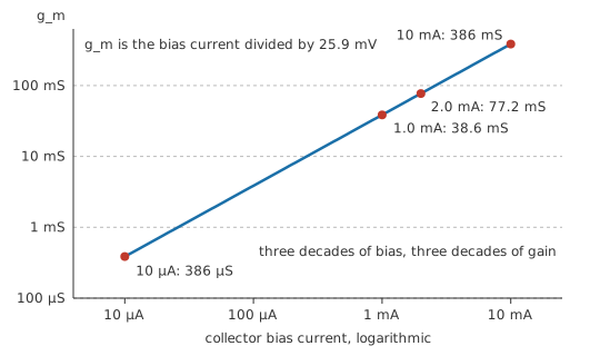
A gain of that sort belongs to an operating point rather than to a part number. For a bipolar transistor the transconductance is the collector current divided by the thermal voltage — about 25.9 mV near room temperature. Biased at 1.0 mA, the device presents 38.6 mS. Move the bias to 2.0 mA and the transconductance becomes 77.2 mS, in exact proportion. The same physical transistor, ordered from the same reel, is a different VCCS at every bias current, which is why biasing gets a lesson of its own and why datasheets quote small-signal parameters against a stated test condition.
The model rests on a linearisation, so it describes the device's response only to excursions small enough that the curve it sits on can be treated as its tangent, and for a bipolar transistor that means signal swings well under the thermal voltage. It is silent, too, about the DC conditions that put the device there — a small-signal model of a saturated transistor is arithmetic about a situation that does not exist.
Feedback is what makes the huge, badly controlled gains usable. An op-amp's open-loop voltage gain is a large number known only to within a factor of several, drifting with temperature and falling steadily with frequency. Wrapping resistors around it trades almost all of that gain for a closed-loop gain set by a resistor ratio, which is stable, predictable and cheap. The analysis that proves this works is ordinary linear circuit analysis performed on a VCVS, which is the abstraction doing real design work rather than sitting in a textbook.
In SPICE and its descendants the four types are separate element letters: E is a voltage-controlled voltage source, G a voltage-controlled current source, H a current-controlled voltage source, and F a current-controlled current source. The voltage-controlled pair name their controlling nodes directly. The current-controlled pair instead name a voltage source to sense the controlling current through, which is why netlists so often contain a zero-volt source inserted for no reason other than to act as an ammeter.
A simulator will let those elements get away with a great deal. A netlist VCVS has unlimited output swing, zero output impedance and no bandwidth limit; a netlist VCCS will force its current into an open circuit. Build a system-level block out of them and the simulation reports gain in regions where the real part has none, and reports it confidently. Two ideal voltage sources connected in parallel produce a singular matrix and a convergence failure instead. Plain elements suit system-level behaviour and a hybrid-pi model suits hand analysis, but wherever the answer depends on a limit, only a full device model will supply it.
Common mistakes
- "Kill all the sources" — the deactivation step in superposition and in the Thévenin-resistance shortcut applies to independent sources only. Dependent sources stay in the circuit and keep obeying their rule in every sub-analysis.
- Treating the gain as a property of the part number — a transistor's transconductance is set by the current you bias it at, so the same device at a tenth of the current has a tenth of the transconductance.
- A gain quoted without its unit — two of the four gains are pure numbers and two are not. The unit is often the only thing in a specification that tells you which of the four you are looking at.
- Forgetting the constraint equation. A dependent source adds an unknown to a nodal or mesh analysis as well as a source. Express its controlling variable in terms of the node voltages or loop currents before solving, or the equation count will not balance.
- A circle drawn where a diamond belongs — on a hand-drawn schematic the outline is the only thing separating a fixed value from a computed one, and a reader who misses it will deactivate the source at the first opportunity.
- Expecting the model to fail the way the device does. Ideal controlled sources have no saturation, no bandwidth limit and no noise. They will happily report an answer for an operating region the real part cannot reach.
Frequently asked questions
What is a dependent source?
A voltage or current source whose value is set by a voltage or current elsewhere in the same circuit, rather than being fixed. It is drawn as a diamond, and it is the standard building block for modelling amplifying devices.
What is the difference between a dependent and an independent source?
An independent source imposes a fixed value on the circuit. A dependent source has no value of its own — it delivers a gain multiplied by some controlling voltage or current found somewhere else in the same circuit.
Why is a dependent source not deactivated in superposition?
Deactivation removes the external excitations one at a time so their individual contributions can be added. A dependent source is not an excitation; it is an internal constraint that must hold in every sub-circuit, so it stays active throughout.
Is a circuit containing dependent sources still linear?
Yes, provided each dependent source's output is a constant times its controlling variable. That relationship is linear, so superposition, Thévenin, Norton, nodal and mesh analysis all still apply.
What are the gain units of the four types?
A VCVS has a dimensionless voltage gain and a CCCS a dimensionless current gain. A VCCS has a transconductance in siemens, and a CCVS a transresistance in ohms.
Which SPICE elements represent controlled sources?
E is a voltage-controlled voltage source, G a voltage-controlled current source, H a current-controlled voltage source and F a current-controlled current source. The F and H elements sense their controlling current through a named voltage source.