
Quick Answer
Mesh analysis solves a planar circuit by assigning a circulating current to each mesh, meaning each window of the drawing, and writing Kirchhoff's voltage law once round each one. A branch on the outer rim carries a single mesh current, while a branch shared by two meshes carries their difference. Solving the simultaneous equations yields every branch current.
Intuition
One circulating current per window
A single loop has one current in it, and Kirchhoff's voltage law round that loop is one equation in one unknown. Join a second loop to the first so the two share a branch, and the arrangement stops being that convenient. The shared branch lies on both routes, and the current in it is not the current in either loop's outer part.
Mesh analysis restores the convenience by inventing something that is not there. Look at the schematic as a drawing and find its windows: the regions of the page with components round the edge and nothing crossing them. One window is one mesh. Now imagine a current going round and round inside each window, all of them turning the same way, clockwise by the usual convention. They are bookkeeping quantities. The circuit itself has no current running round and round anywhere in it.
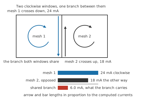
Everything then follows from where a branch sits. A branch on the outer rim of the drawing borders one window only, so it carries that window's circulating current alone. A branch between two windows lies on the edge of both, and since both circulate the same way round their own window, they run through that shared branch in opposite directions.
Such a branch therefore carries the difference. Suppose the left window comes out at 24 mA and the right one at 18 mA: the branch between them carries 6.0 mA, going the way the left one turns. Every real current in the circuit is recovered like that once the mesh currents are known, by reading one straight off the rim or subtracting a pair in the middle.
Practitioner
Setting the equations down and solving them
None of the steps below takes long. One word in them needs pinning down first: a branch is a stretch of circuit running between two junctions and carrying one current along its whole length, whether that stretch holds a single resistor or several components in a line with nothing joining on between them.
- Satisfy yourself that the schematic can be drawn with no wire crossing another, then mark its windows. Each window is a mesh.
- Draw a circulating current in every mesh, all of them clockwise.
- Walk each mesh in that direction, writing one term per element crossed, and set the terms to zero. The sign of each term comes from which terminal you meet first: a rise if you enter at the lower-potential end, a fall if you enter at the higher.
- In a branch shared with a neighbouring mesh, the current is your own mesh current minus the neighbour's.
- Solve the set.
- Convert back to branch currents. Rim branches carry one mesh current; shared branches carry a difference.
Most of the terms come from a current and a resistance:
and the terms of one mesh close on the sources it contains:
The library entry is a loop with three voltages in it, which is the case worked below. A mesh may hold any number of them. The general statement has to be made in words — the signed voltages round a closed loop sum to zero — because an expression is fixed at the number of terms it was written with, and mesh analysis therefore has no formula of its own to look up.
Step 4 is the one that goes wrong most often. Write the shared branch's term with your own mesh current alone and the neighbour drops out entirely, leaving a set of equations that describes two separate circuits.
Worked example — Two supply rails meeting at one node
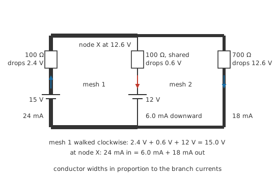
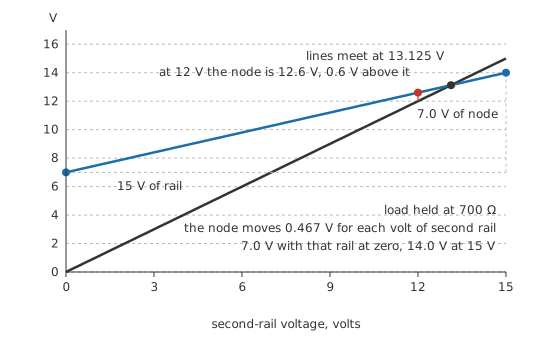
A 15 V rail reaches node X through 100 Ω. A second rail, at 12 V, reaches the same node through its own 100 Ω. From X a load of 700 Ω runs down to the common rail. Three branches meet at X, and the drawing has two windows: mesh 1 bounded by the two supply branches, mesh 2 by the second supply branch and the load.
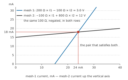
Walk mesh 1 clockwise, up the first supply branch and down the second. Its resistive terms are 100 Ω carrying the mesh 1 current and 100 Ω carrying the difference, so the coefficient of the mesh 1 current is 200 Ω and the coefficient of the mesh 2 current is 100 Ω negated. The two sources are met in opposition, one as a rise and one as a fall, which leaves 3.0 V on the right-hand side.
Mesh 2 runs up the shared branch and down the load. Its own coefficient is 800 Ω, the shared resistance appears negated again, and the second source is now met as a rise, so its right-hand side is 12 V.
The pair solves to 24 mA and 18 mA.
The branch currents come out of those two. The first supply branch is on the rim and carries 24 mA; the load is on the rim and carries 18 mA. The shared branch takes the difference, 6.0 mA, flowing from X down into the second source, so that rail is taking current in.
The result comes with its own checks. Round mesh 1 the drops are 2.4 V, 0.6 V and the second source's own 12 V, which together come to 15.0 V, the first rail's figure. At node X the arriving 24 mA leaves as 6.0 mA and 18 mA, with the node standing at 12.6 V.
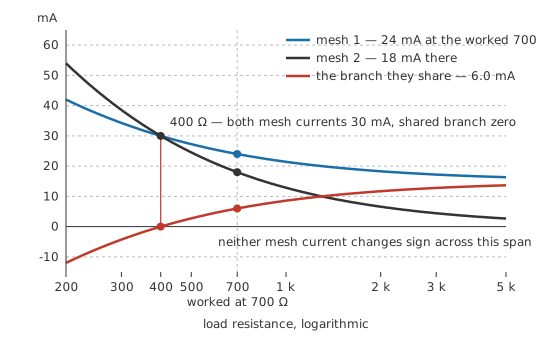
A mesh current can come out negative, and that answer stands as it is. It reports circulation running anticlockwise in that window, and every branch expression built from it keeps its validity, signs and all. Sign errors tend to come from the opposite instinct: rubbing the arrow out and starting the derivation again.
Before reaching for any of this, try reduction by series and parallel steps. A network that collapses gives up its currents through arithmetic alone, without a simultaneous equation anywhere. Mesh analysis is for the ones that refuse to collapse, and unlike the delta-wye swap it asks nothing of the topology beyond a drawing without crossings.
Engineer
The coefficient matrix and its exceptions
A current circulating round a closed window enters every node on that window and leaves it again, so Kirchhoff's current law holds at every node before a single equation exists. That is the justification for the device: the node equations are settled by construction, and only the loop equations remain.
Every coefficient in a mesh equation is a resistance, because every resistive term in it is a current multiplied by one:
Set the worked example's two equations side by side and the coefficients fall into a pattern. Along the diagonal sit 200 Ω and 800 Ω, each the sum of every resistance round its own mesh. The shared 100 Ω appears off the diagonal, negated, in both positions. On the right stand 3.0 V and 12 V, the net source rise met on each walk.
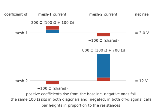
Filling that array off the drawing, with no walk written down, is called the inspection method. It is a shortcut with conditions: resistances and independent voltage sources only, every mesh current clockwise, and then
- row k, column k is the self-resistance of mesh k, the sum of all resistances on its boundary;
- row k, column j is the sum of the resistances meshes k and j have in common, negated;
- the right-hand entry of row k is the net rise from the sources in mesh k, in the direction of travel.
The minus sign, and its presence in both positions, comes out of the geometry. The shared resistance lies on the boundary of both meshes, and the two clockwise currents pass through it in opposite senses whichever mesh you walk, so each equation subtracts the neighbour by the same amount. The resulting symmetry doubles as a proofreading test: a lopsided array holds a slip, or a mesh current that was never drawn clockwise.
Those conditions are easy to lose. A dependent source contributes a term built from a current or voltage elsewhere in the circuit, landing in one row with no partner in the other, and the symmetry goes with it. Linearity is assumed throughout as well, since every element needs a constant to put in the array, and a diode or a filament lamp offers none. Either way the shortcut is gone, and the circuit is walked mesh by mesh or linearised about an operating point first.
A current source in a shared branch
An ideal current source fixes the current through itself and lets its terminal voltage be whatever the surrounding circuit demands. That voltage is an unknown with nothing to express it in terms of, so its branch has no KVL term and the mesh containing it has no equation.
Where the source sits decides the remedy. On the rim it borders one mesh and fixes that mesh's current outright, and the known value enters the neighbouring equations as a constant. Between two meshes it fixes only the difference. Treat the pair as one larger loop — a supermesh — whose boundary runs round the outside and never enters the shared branch: KVL round that boundary gives one equation, the source's own current the other.
Worked example — A current source between two windows
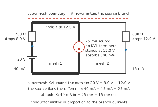
The left branch holds a 20 V source in series with 200 Ω, running up to node X. The shared branch is a current source drawing 25 mA from X down to the common rail. The right branch is 800 Ω, from X back down to that rail.
The constraint comes first, and it is written down rather than derived. The shared branch is crossed downward by mesh 1 and upward by mesh 2, so the mesh currents differ by 25 mA.
For the second equation, walk the outside of the pair — up through the source and 200 Ω, across the top, down 800 Ω — so the shared branch never appears. A rise of 20 V stands against one drop weighted by 200 Ω and another by 800 Ω.
That pair solves at once: 40 mA in the left mesh, 15 mA in the right. The left branch drops 8.0 V, putting X at 12.0 V.
The source's own voltage arrives last, out of the equation that could not be written. Round mesh 2, crossing the source upward has to balance the 12.0 V dropped in the right branch, so the source stands at 12.0 V and absorbs 300 mW.
When a circuit will not lie flat
A mesh is a window in a drawing, so the circuit has to be drawable flat with no branch crossing another before any of this is defined. Networks that can be are called planar, and most schematics are: a crossing on the page is often an artefact of layout that a rearrangement removes.
A few resist rearranging. Five nodes each joined directly to all four of the others is the standard example: no flat arrangement avoids a crossing, so the network has no windows at all. Nodal analysis carries no such condition, since a node is a feature of the connections rather than of the picture.
Where windows do exist, how many is settled by the connections rather than the layout. A connected network of B branches and N nodes has B − N + 1 independent loop equations, and on a planar drawing the windows are exactly that many, so two people who lay the same netlist out differently reach the same answers. Kirchhoff's current law supplies the other N − 1, and the B element relations complete the set.
Professional
Counting equations before you choose
Which method leaves fewer unknowns
For a connected network of B branches and N nodes, mesh analysis produces B − N + 1 equations and nodal analysis produces N − 1. Set one against the other and mesh wins whenever B is smaller than 2N − 2, which is to say on circuits with many nodes strung out along relatively few branches. A long cascade of stages or a ladder has plenty of nodes and few windows, and mesh analysis is the shorter job there. Circuits with a handful of nodes and a crowd of branches between them go the other way: a supply rail with twelve loads across it has two nodes and thirteen branches, which is one node equation against twelve mesh equations.
The first worked circuit falls on the nodal side of that line, and it is fairer to say so. Three branches and two nodes give two mesh equations against a single node equation, and anyone solving it for its own sake would write the node equation. It was chosen to show the shared-branch step on numbers small enough to check by hand.
The kind of source matters as much as the count. Voltage sources are free in a mesh equation, where they sit as ordinary terms, while a voltage source between two non-reference nodes forces nodal analysis into a supernode. Current sources are the reverse: free in a node equation, and the reason supermeshes exist at all. A circuit thick with voltage sources and thin on current sources leans towards mesh even where the counts are close, and source transformation will move a circuit from one camp to the other before either method starts.
Auditing a solution costs one pass
A solved circuit can be audited rather than re-derived, and the power relations do the work:
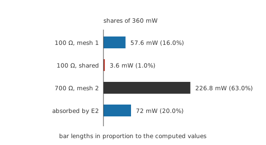
In the first circuit the 15 V rail delivers 360 mW. The three resistances take 57.6 mW, 3.6 mW and 226.8 mW, and the second rail, receiving current instead of supplying it, absorbs a further 72 mW. Those four come to 360 mW, matching what was delivered. An audit of that kind catches a dropped term or a sign error; a second run through the same algebra tends to reproduce both.
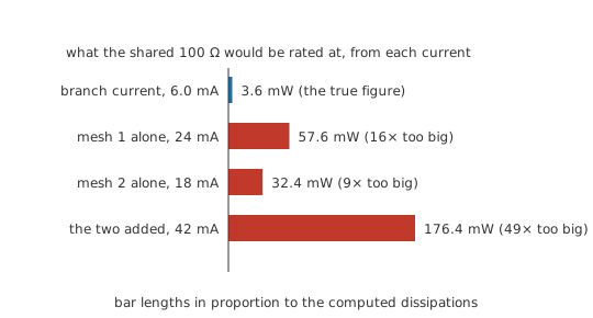
Dissipation figures come off branch currents, and a mesh current is the wrong quantity to put into them. The resistance in the shared branch here carries 6.0 mA and turns 3.6 mW into heat; specified from either mesh current instead, it would be bought many times larger than it needs to be.
What a simulator solves instead
SPICE and its descendants do not use mesh analysis. They use modified nodal analysis: node voltages as the unknowns, plus one extra unknown current for every element whose branch relation cannot be written as a current in terms of node voltages, ideal voltage sources first among them.
The reason has more to do with bookkeeping than with mathematics. A netlist is a list of elements and the nodes they join, and each element can be stamped into the matrix on its own, in any order, with no knowledge of the rest of the circuit. Identifying meshes is a separate problem in graph theory that has to be solved before one equation can be written, and it fails outright on a non-planar netlist. Modified nodal analysis also extends without redesign to nonlinear elements, to the time domain and to frequency sweeps.
How the cost grows
Solving n simultaneous equations by straight Gaussian elimination costs work proportional to n cubed, which is why the choice of method is more than a question of neatness. Real circuit matrices are sparse — a mesh borders only its immediate neighbours, so most entries are zero — and sparse solvers exploit that to stay well below the cube. Hand work meets its ceiling much earlier: two unknowns are comfortable, three are a chore, four are where most people stop. When the question is one current in one branch of a large network rather than all of them, Thévenin's theorem or superposition often reaches it for less work than either systematic method.
Common mistakes
- Adding the two mesh currents in a shared branch instead of subtracting them. Both are clockwise in their own window, so they cross the branch they share in opposite directions. Subtract, taking the current of the mesh you are working in first.
- "A mesh current is the current in that wire." True only on the rim. Any branch bordering two windows carries a combination, and reading a mesh current off as a branch current is how a correctly solved circuit still yields wrong answers.
- Choosing a direction mesh by mesh. Mixing clockwise and anticlockwise windows does not make the answers wrong, but it destroys the sign pattern that lets the array be written by inspection and tested for symmetry.
- A region of the drawing with a component crossing it. That is two windows. Meshes are the smallest closed regions the drawing leaves, and treating a larger loop as one mesh loses an equation from the set.
- Writing a KVL term for a branch containing a current source. There is nothing to write, because the source's voltage stays unknown until the rest is solved. Combine the two meshes into a supermesh and take the second equation from the source's own current.
- Power ratings taken from mesh currents. A mesh current is a bookkeeping figure; the heat in a shared element follows the branch current, which can be very much smaller. Convert back to branches before sizing anything.
Frequently asked questions
Do all the mesh currents have to circulate the same way?
The mathematics is indifferent to it, and the answers come out identical either way. A uniform choice buys the sign pattern: with every mesh clockwise, every off-diagonal coefficient is negative and the array is symmetric, so it can be written by inspection and checked at a glance. The only effect of mixing them is the loss of that pattern.
Is a mesh current something I could measure?
No instrument reads one. It is introduced so that Kirchhoff's current law is satisfied automatically, since a current circulating round a closed window neither accumulates nor disappears at any node it passes. Only the branch currents recovered afterwards correspond to what a meter clipped into the circuit would report.
How do I know I have found every mesh?
Count the branches and the nodes and compare. A spanning tree reaching every node uses N minus 1 branches and closes no loop at all; each of the remaining branches closes exactly one, which puts the count at B minus N plus 1. A drawing showing fewer windows than that is not yet a planar drawing of the circuit, and rearranging it to remove a crossing will bring the missing window out.
What if two meshes share more than one branch?
Add the shared resistances together. The off-diagonal coefficient is the total resistance the two meshes have in common, whether that sits in one branch or in three, and it is still negated and still appears in both rows.
Does the method work on AC circuits?
Yes, with impedances in place of resistances and phasor values in place of the source figures. The array keeps its shape, self-impedances on the diagonal and shared impedances negated off it, while the arithmetic becomes complex instead of real. Capacitors and inductors change no topology, so the meshes are counted exactly as before.